

GPU-Accelerated Land Use Land Cover Classification#
Working with satellite imagery at scale quickly exposes the limitations of CPU-bound workflows. A single Sentinel-2 tile spans gigabytes and assembling a season’s worth of acquisitions means streaming dozens of those tiles, masking pixels covered by clouds, and compositing them before you can even think about training a model. Processing data of such scale on CPUs means hours of preprocessing before training, making GPUs an attractive solution to accelerate the workflow.
Due to the parallel nature of satellite data, GPUs can dramatically accelerate the compute-bound stages of a machine learning workflow. RAPIDS libraries like cuDF and cuML with the help of other libraries like Dask and Xarray map operations to CUDA kernels, so feature derivation and tree training execute across thousands of cores at once. By keeping the samples in GPU memory between those stages, we avoid the overhead of shuffling data back and forth across the host and device memory. Not every stage benefits equally, and it is worth being precise about which do: streaming scenes from a remote catalogue is bound by network and disk throughput, while model training and inference are compute-bound and are where the GPU earns its usage.
This notebook establishes a end-to-end workflow to train a classification model on satellite imagery. We start by streaming Sentinel-2 imagery from Microsoft Planetary Computer into a Dask-CUDA cluster, using Dask backed xarray to clean and aggregate the rasters. We then move the samples on device to train a cuML random forest and finish by writing predictions straight back to Cloud-Optimized GeoTIFFs, ready for validation and sharing.
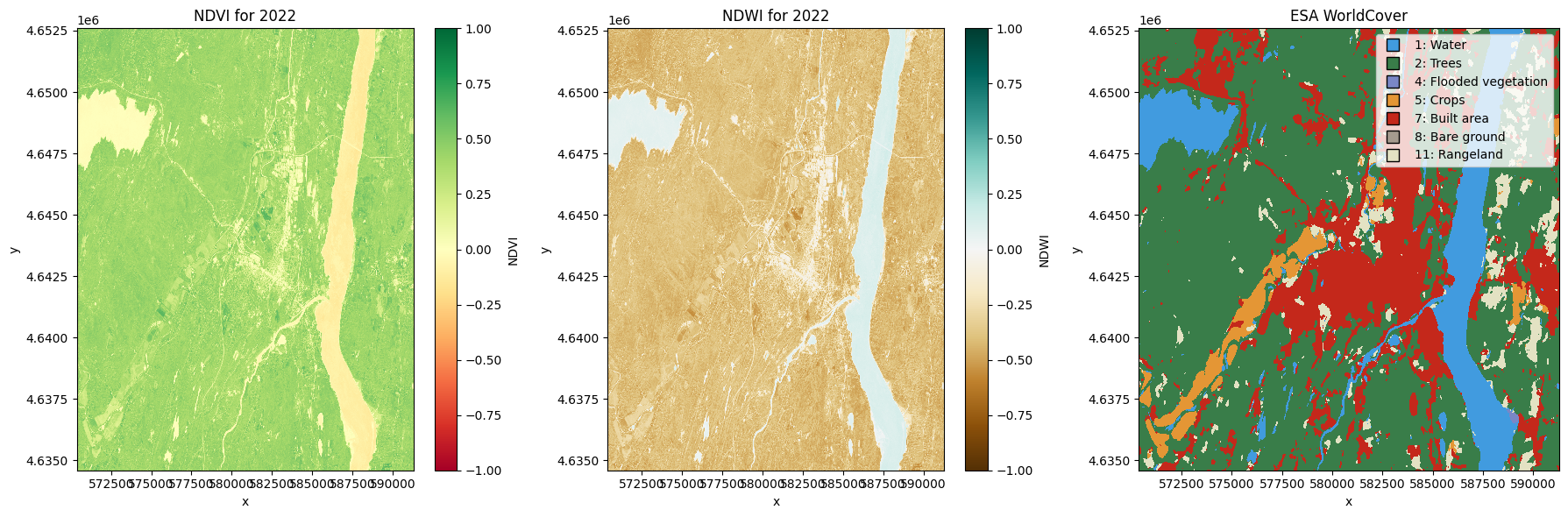
For this workflow, we use two open and freely available data sources as features and labels, downloaded from Microsoft Planetary Computer. Sentinel-2 Level-2A imagery supplies 10 m multispectral observations (B02, B03, B04, B08 are the 10 metre bands that correspond to blue, green, red and near-infrared wavelengths) annually with a 5 day revisit frequency, which we condense into cloud-free yearly composites and enrich with indices like NDVI and NDWI for the year 2022. ESA WorldCover provides annual 10 m land-cover labels, with its 2023 release reflecting the landscape from 2022, giving us labels for supervised training. Together they provide the coverage and scale to illustrate the benefits of using GPUs for this task.
The machine learning use case illustrated in this notebook, Land use and land cover (LULC) classification, is the task of labelling each pixel in an image according to the surface type it represents. Typical labels include water, trees, crops, built areas, bare ground, and rangeland. These maps help planners monitor urban growth, estimate crop acreage, or track ecosystem change.
The next two sections cover what you need installed and what kind of machine to run it on.
Before You Begin#
What this notebook uses#
Three RAPIDS libraries do the GPU work and you do not need a full RAPIDS installation for this workflow:
cuML trains the
RandomForestClassifierand scores it.cuDF holds the flattened pixel samples as GPU DataFrames, which cuML consumes directly with no host round-trip.
Dask-CUDA provides
LocalCUDACluster, which parallelises Stage 1 across the GPUs on the machine.
Around those sits a geospatial stack that feeds them. These are ordinary PyData packages rather than RAPIDS ones, and the handoff between the two worlds happens through Xarray:
Package |
Role |
|---|---|
|
Query the STAC catalogue and lazily load matching scenes into an Xarray/Dask cube |
|
Raster I/O, reprojection, and CRS handling |
|
Read the AOI polygons and project them into UTM |
|
Persist the annual composites between stages |
|
Adds the |
|
Write the final Cloud-Optimized GeoTIFF |
You will also need a GeoJSON defining your areas of interest (one is bundled with this example, see Step 1) and network access to Microsoft Planetary Computer, which serves both the Sentinel-2 imagery and the WorldCover labels without requiring an account. Writing the output COG to S3 is optional.
Where this runs#
Everything below runs on a single machine with one or more NVIDIA GPUs. Stage 1 starts a LocalCUDACluster, which launches one Dask worker per visible GPU on that same machine.
If you need to get to such a machine first, these guides cover it:
Dask-CUDA and
LocalCUDACluster- configuration options, pinning specific GPUs, memory limitscloud VMs: AWS EC2, Azure VM, GCP Compute Engine
Adapting this notebook to a multi-node cluster is also an option, see the deployment documentation for more information
How to size the machine#
The figures quoted throughout this notebook were measured on a dual-socket workstation with 2× Intel Xeon E5-2698 v4 (40 cores / 80 threads), 503 GB of RAM, and 8× NVIDIA Tesla V100-SXM2 with 32 GB of VRAM each.
You do not need a machine that size. Training peaks at 1.83 GB of VRAM and inference at roughly 2.3 GB, both on a single device, so any modern NVIDIA GPU with 8 GB or more runs Stages 2 and 3 comfortably. Additional GPUs only matter to Stage 1 and more visible devices means more Dask workers streaming and compositing scenes in parallel.
Host RAM is the real constraint. The raw multi-scene stack peaks at roughly 44 GB during Stage 1, scaling with how many scenes your AOI and date range pull in. Once compositing collapses it to annual medians, the data on disk is only a fraction of that size. Size your RAM to the scene stack, and do not assume you need a multi-GPU node.
Creating the environment#
The environment.yml shipped next to this notebook pins the packages listed above:
conda env create -f environment.yml
conda activate rapids-lulc
python -m ipykernel install --user --name rapids-lulc
Substitute mamba for conda if you prefer. Once the kernel is installed, select rapids-lulc from the Jupyter kernel picker before running any cells below.
import dataclasses
import gc
import json
import pickle
from pathlib import Path

import boto3
import cudf
import cupy as cp
import cupy_xarray  # noqa: F401  activates the .cupy accessor
import geopandas as gpd
import matplotlib.pyplot as plt
import numpy as np
import pandas as pd
import planetary_computer
import pyproj
import rasterio
import rioxarray  # noqa: F401  activates the .rio accessor
import seaborn as sns
import stackstac
import xarray as xr
from cuml.ensemble import RandomForestClassifier
from cuml.metrics import accuracy_score
from dask.distributed import Client as DaskClient
from dask.distributed import progress, wait
from dask_cuda import LocalCUDACluster
from matplotlib.colors import BoundaryNorm, ListedColormap
from pystac_client import Client
from rio_cogeo.cogeo import cog_translate
from rio_cogeo.profiles import cog_profiles
from shapely.ops import transform
from sklearn.metrics import classification_report, confusion_matrix, f1_score
from stackstac.raster_spec import RasterSpec
Stage 1 · Ingest and Prepare Training Data#
We begin by getting the raw ingredients into a form we can model on. That means streaming Sentinel-2 scenes and WorldCover labels straight from the Planetary Computer, reprojecting them onto a common grid, and reshaping them into chunk sizes that Dask can scatter across its workers. The goal is to build clean yearly composites and companion label layers once, persist them as Zarr stores, and avoid recomputing expensive preprocessing later in the notebook.
1. Set Workspace Paths and Parameters#
Run this cell to lock in the project-wide constants the pipeline needs: where to find your AOI GeoJSON, which Sentinel-2 bands and WorldCover assets to request, how to chunk raster stacks, and where to stage intermediate outputs. Update the paths and S3_BUCKET/S3_PREFIX now so the rest of the notebook writes to the right locations. Confirm the directories exist (the code creates any missing output folders for you) and keep the date range and cloud filter aligned with the scenes you plan to process.
This example trains on two areas of interest from 2022, totalling roughly 974 km². They are supplied by aoi_combined.geojson, which can be downloaded alongside this notebook. Point AOI_GEOJSON at that file to reproduce the results below without drawing anything yourself. To use your own areas instead, Step 3 walks through creating a GeoJSON on geojson.io.
AOI |
Extent |
Area |
UTM zone |
Dominant cover |
|---|---|---|---|---|
Minneapolis, MN |
W −93.42, S 44.85, E −93.09, N 45.06 |
606 km² |
EPSG:32615 |
Built area |
Hudson Valley, NY |
W −74.15, S 41.86, E −73.90, N 42.02 |
368 km² |
EPSG:32618 |
Trees, water, crops and rangeland |
An earlier version of this example trained on the urban AOI alone, where roughly 85% of pixels are Built area. The resulting model reported a flattering 90.8% accuracy while never once predicting flooded vegetation, crops, or bare ground. Adding a land-cover diverse AOI with the Catskills, the Hudson River and the Ashokan Reservoir supplies the classes the AOI from the urban areas was missing. We revisit the consequences of this in Stage 2.
AOI_GEOJSON = Path("<path to your AOI GeoJSON file>")
FEATURES_ZARR = Path("<desired path for the features zarr store>")
MODEL_PATH = Path("<desired path for the model file ending with .pkl>")
INFERENCE_OUTPUT_DIR = Path("<desired path for the inference output directory>")
AWS_REGION = "<your AWS region>"
S3_BUCKET = "<your S3 bucket name>"
S3_PREFIX = "lulc"
MODEL_PATH.parent.mkdir(parents=True, exist_ok=True)
# General configuration / outputs
DATE_RANGE = ("2022-01-01", "2022-12-31")
MAX_CLOUD_FILTER = (
    50  # Set this value higher to fetch more scenes with higher cloud cover
)
S2_ASSETS = ["B02", "B03", "B04", "B08", "SCL"]

TARGET_RESOLUTION = 10
STACK_CHUNKS = {"time": 1, "band": 1, "y": 2048, "x": 2048}

WORLDCOVER_COLLECTION = "io-lulc-annual-v02"
WORLDCOVER_ASSET = "data"

FEATURES_ZARR.mkdir(parents=True, exist_ok=True)
INFERENCE_OUTPUT_DIR.mkdir(parents=True, exist_ok=True)
MODEL_PATH.parent.mkdir(parents=True, exist_ok=True)

CATALOG_URL = "https://planetarycomputer.microsoft.com/api/stac/v1"

BANDS = ["B02", "B03", "B04", "B08"]
ALL_FEATURES = ["B02", "B03", "B04", "B08", "NDVI", "NDWI"]
NODATA_VALUE = 0
VALID_CLASSES = [1, 2, 4, 5, 7, 8, 11]

COG_PROFILE = cog_profiles.get("deflate")
s3_client = boto3.client("s3", region_name=AWS_REGION)
2. Launch a Dask-CUDA Cluster#
Start the local Dask-CUDA cluster now so every downstream step can submit work through the distributed client. Run this cell and confirm the dashboard link appears. LocalCUDACluster starts one worker per visible GPU; if you need to pin workers to specific devices or change memory limits, modify its arguments before proceeding.
cluster = LocalCUDACluster()
client = DaskClient(cluster)
client
/raid/jjayabaskar/gis12/lib/python3.12/site-packages/distributed/node.py:187: UserWarning: Port 8787 is already in use.
Perhaps you already have a cluster running?
Hosting the HTTP server on port 45991 instead
  warnings.warn(
Client
Client-2333aeb6-804d-11f1-a199-d8c49778cfa7
| Connection method: Cluster object | Cluster type: dask_cuda.LocalCUDACluster |
| Dashboard: http://127.0.0.1:45991/status |
Cluster Info
LocalCUDACluster
e186339d
| Dashboard: http://127.0.0.1:45991/status | Workers: 8 |
| Total threads: 8 | Total memory: 503.77 GiB |
| Status: running | Using processes: True |
Scheduler Info
Scheduler
Scheduler-b978fefe-1535-41a9-9f5d-2b08dcdf9570
| Comm: tcp://127.0.0.1:38355 | Workers: 0 |
| Dashboard: http://127.0.0.1:45991/status | Total threads: 0 |
| Started: Just now | Total memory: 0 B |
Workers
Worker: 0
| Comm: tcp://127.0.0.1:42971 | Total threads: 1 |
| Dashboard: http://127.0.0.1:37175/status | Memory: 62.97 GiB |
| Nanny: tcp://127.0.0.1:37415 | |
| Local directory: /tmp/dask-scratch-space/worker-za5lmvuu | |
Worker: 1
| Comm: tcp://127.0.0.1:40007 | Total threads: 1 |
| Dashboard: http://127.0.0.1:46655/status | Memory: 62.97 GiB |
| Nanny: tcp://127.0.0.1:32941 | |
| Local directory: /tmp/dask-scratch-space/worker-f_y63d_z | |
Worker: 2
| Comm: tcp://127.0.0.1:43395 | Total threads: 1 |
| Dashboard: http://127.0.0.1:34291/status | Memory: 62.97 GiB |
| Nanny: tcp://127.0.0.1:36901 | |
| Local directory: /tmp/dask-scratch-space/worker-gfdiyini | |
Worker: 3
| Comm: tcp://127.0.0.1:42363 | Total threads: 1 |
| Dashboard: http://127.0.0.1:46341/status | Memory: 62.97 GiB |
| Nanny: tcp://127.0.0.1:42739 | |
| Local directory: /tmp/dask-scratch-space/worker-kl9csyhp | |
Worker: 4
| Comm: tcp://127.0.0.1:37379 | Total threads: 1 |
| Dashboard: http://127.0.0.1:36469/status | Memory: 62.97 GiB |
| Nanny: tcp://127.0.0.1:32999 | |
| Local directory: /tmp/dask-scratch-space/worker-krgker1d | |
Worker: 5
| Comm: tcp://127.0.0.1:44011 | Total threads: 1 |
| Dashboard: http://127.0.0.1:44051/status | Memory: 62.97 GiB |
| Nanny: tcp://127.0.0.1:37453 | |
| Local directory: /tmp/dask-scratch-space/worker-hnvsz41b | |
Worker: 6
| Comm: tcp://127.0.0.1:41505 | Total threads: 1 |
| Dashboard: http://127.0.0.1:43341/status | Memory: 62.97 GiB |
| Nanny: tcp://127.0.0.1:40005 | |
| Local directory: /tmp/dask-scratch-space/worker-11wn3e7i | |
Worker: 7
| Comm: tcp://127.0.0.1:34901 | Total threads: 1 |
| Dashboard: http://127.0.0.1:41435/status | Memory: 62.97 GiB |
| Nanny: tcp://127.0.0.1:41639 | |
| Local directory: /tmp/dask-scratch-space/worker-x0nzq6pz | |
3. Load and Reproject the Areas of Interest#
Use this cell to validate and prepare your AOI geometries. It reads the GeoJSON configured earlier, checks that a CRS is declared, and builds one entry per polygon. Run it once to produce the aois list, where each entry holds a geometry, its projected bounds, its EPSG code, and a GeoJSON payload that the STAC search reuses.
A short detour on coordinate reference systems#
A coordinate reference system (CRS) is the agreement that turns a pair of numbers into a place on the Earth. Geospatial tools identify them by EPSG code, and for this workflow only two families matter.
EPSG:4326 (often called “WGS 84” or “lat/lon”) expresses positions as degrees of latitude and longitude on an ellipsoid. It is the lingua franca of data exchange - GeoJSON files are assumed to be in it, and every STAC catalogue accepts search geometries in it. What it cannot do is measure. A degree of longitude is about 111 km at the equator and about 79 km at the latitude of Minneapolis, so the same numeric distance means different things depending on where you are. You cannot ask for “10 metre pixels” in a CRS whose units are degrees, and an area computed in square degrees is meaningless.
UTM zones solve that by slicing the world into 60 north-south strips six degrees wide and projecting each onto a flat plane whose units are metres. Their EPSG codes follow a simple pattern: 326 + zone number for the northern hemisphere, 327 + zone number for the southern. Minneapolis sits in zone 15, so it is EPSG:32615; the Hudson Valley sits in zone 18, so it is EPSG:32618. Within a zone, distortion is small enough that a 10 m pixel really is 10 m on the ground, which is exactly what TARGET_RESOLUTION = 10 assumes.
This is why the cell below does two different things with the same geometry. It keeps a 4326 GeoJSON payload to hand to the STAC search, and separately projects the polygon into its own UTM zone to compute the metre-based bounding box that stackstac needs. It also explains why each AOI is handled independently rather than merged: because our two AOIs fall in different zones, there is no single metre-based grid that covers both without stretching one of them. Forcing them into a shared CRS would distort pixel geometry at the edges and inflate the bounding box to span the 1,000 km of empty ground between Minnesota and New York.
Drawing your own AOI#
To create an AOI in GeoJSON format by drawing polygons over a map interactively, use geojson.io. Draw one or more shapes, add a name property to each feature so the notebook can label its outputs, then use Save → GeoJSON and point AOI_GEOJSON at the downloaded file. Keep individual AOIs modest to begin with - a few hundred square kilometres over a year of Sentinel-2 revisits is already tens of gigabytes of imagery to stream.
aoi_gdf = gpd.read_file(AOI_GEOJSON)
if aoi_gdf.crs is None:
    raise ValueError("AOI GeoJSON must declare a CRS.")
aoi_gdf = aoi_gdf.to_crs(4326)

# Build one entry per polygon. Each AOI keeps its OWN UTM zone and bounding box,
# so polygons in different zones (Minneapolis = 15, Hudson Valley = 18) are each
# projected correctly instead of being forced into one oversized shared extent.
aois = []
for i, row in aoi_gdf.iterrows():
    geom = row.geometry
    name = row.get("name", f"aoi_{i}")
    centroid = geom.centroid
    utm_zone = int((centroid.x + 180) // 6) + 1
    epsg = int(f"326{utm_zone:02d}") if centroid.y >= 0 else int(f"327{utm_zone:02d}")
    geojson = json.loads(gpd.GeoSeries([geom], crs=4326).to_json())["features"][0][
        "geometry"
    ]
    project = pyproj.Transformer.from_crs(4326, epsg, always_xy=True).transform
    bounds = tuple(transform(project, geom).bounds)
    aois.append(
        {
            "name": name,
            "slug": str(name).replace(" ", "_"),
            "geom": geom,
            "geojson": geojson,
            "epsg": epsg,
            "bounds": bounds,
        }
    )
for a in aois:
    print(
        f"{a['name']:>16} | EPSG {a['epsg']} | bounds {tuple(round(b) for b in a['bounds'])}"
    )
     Minneapolis | EPSG 32615 | bounds (466811, 4966291, 492914, 4989701)
   Hudson Valley | EPSG 32618 | bounds (570373, 4634582, 591299, 4652582)
4. Fetch Sentinel-2 tiles for each AOI#
Search the Planetary Computer STAC API for Sentinel-2 Level-2A scenes that overlap each AOI, match the configured date window, and meet the cloud threshold. Run this cell to pull the items, guard against empty results, and build a lazily-loaded raster stack with stackstac per AOI. Each stack is clipped to its own AOI bounds, resampled to the target resolution, and chunked for parallel processing.
stac = Client.open(CATALOG_URL, modifier=planetary_computer.sign_inplace)

# Fetch, clip, resample and persist a stack for each AOI. Each AOI is searched
# with its own 4326 geometry but stacked onto its own UTM grid.
for a in aois:
    items = list(
        stac.search(
            collections=["sentinel-2-l2a"],
            intersects=a["geojson"],
            datetime=f"{DATE_RANGE[0]}/{DATE_RANGE[1]}",
            query={"eo:cloud_cover": {"lt": MAX_CLOUD_FILTER}},
        ).items()
    )
    if not items:
        raise ValueError(f"No Sentinel-2 scenes for AOI '{a['name']}'.")

    stack = (
        stackstac.stack(
            items,
            assets=S2_ASSETS,
            bounds=a["bounds"],
            resolution=TARGET_RESOLUTION,
            epsg=a["epsg"],
            chunksize=(200, 1, 1024, 1024),
            fill_value=np.nan,
            rescale=False,
            properties=["datetime"],
            # Nearest neighbour is stackstac's default; we state it explicitly
            # because SCL is a 20 m categorical band and interpolating class
            # codes on the way to 10 m would invent values that mean nothing.
            resampling=rasterio.enums.Resampling.nearest,
        )
        .astype("float32")
        .sortby("time")
    )
    stack = stack.assign_coords(band=S2_ASSETS[: stack.sizes["band"]])
    a["stack"] = stack.persist()
    print(f"{a['name']}: {len(items)} scenes -> stack {a['stack'].shape}")

aois[0]["stack"]
Minneapolis: 92 scenes -> stack (92, 5, 2342, 2611)
Hudson Valley: 84 scenes -> stack (84, 5, 1801, 2093)
<xarray.DataArray 'stackstac-0428415431f44c8b1dd9346ca21b32ec' (time: 92,
                                                                band: 5,
                                                                y: 2342, x: 2611)> Size: 11GB
dask.array<asarray, shape=(92, 5, 2342, 2611), dtype=float32, chunksize=(92, 1, 1024, 1024), chunktype=numpy.ndarray>
Coordinates:
  * time                 (time) datetime64[ns] 736B 2022-01-06T17:07:09.02400...
  * band                 (band) <U3 60B 'B02' 'B03' 'B04' 'B08' 'SCL'
  * y                    (y) float64 19kB 4.99e+06 4.99e+06 ... 4.966e+06
  * x                    (x) float64 21kB 4.668e+05 4.668e+05 ... 4.929e+05
    id                   (time) <U54 20kB 'S2B_MSIL2A_20220106T170709_R069_T1...
    title                (band) <U29 580B 'Band 2 - Blue - 10m' ... 'Scene cl...
    gsd                  (band) float64 40B 10.0 10.0 10.0 10.0 20.0
    proj:bbox            object 8B {399960.0, 509760.0, 5000040.0, 4890240.0}
    common_name          (band) object 40B 'blue' 'green' 'red' 'nir' None
    center_wavelength    (band) object 40B 0.49 0.56 0.665 0.842 None
    full_width_half_max  (band) object 40B 0.098 0.045 0.038 0.145 None
    epsg                 int64 8B 32615
Attributes:
    spec:        RasterSpec(epsg=32615, bounds=(466810, 4966290, 492920, 4989...
    crs:         epsg:32615
    transform:   | 10.00, 0.00, 466810.00|\n| 0.00,-10.00, 4989710.00|\n| 0.0...
resolution: 10progress([a["stack"] for a in aois])
Persisting the stack up front forces Dask to scatter chunks across every available worker before we start feature engineering. If we wait until the first compute call, the scheduler will place most of the chunks onto a single worker to avoid shuffle overhead, which in turn runs the risk of running out of memory. By persisting the data now, we keep it evenly distributed for the rest of the pipeline.
5. Prepare Daily Spectral Composites#
Satellite imagery is usually captured in the form of tiles, a specific image captured by the satellite corresponding to a certain area, specified in the tile extent. In the previous step, we captured all the tiles that intersect with our AOI for all dates in 2022. However, there might be multiple tiles that intersect with our AOI captured on a specific date. These tiles also occasionally do intersect in area, so before calculating an annual median value for each pixel, we group this data by unique capture dates and use the median value for band-wise reflectance where tiles overlap.
Sentinel-2 tiles also include a special band called the Sentinel-2 Scene Classification Layer (SCL), which tags each pixel with a surface or atmospheric class inferred from the Level-2A processing chain. It distinguishes nodata (0), saturated or defective pixels (1), dark areas (2), cloud shadow (3), vegetation (4), bare soils (5), water (6), cloud probabilities from low to high (7–9), thin cirrus (10), and snow or ice (11). Using SCL lets you mask out cloudy or otherwise unreliable observations before aggregating daily composites, so only the clear-sky land pixels (classes 4–6 and 11) contribute to the summaries.
In the following steps, we assign a daily date coordinate, split out the Sentinel-2 Scene Classification Layer (SCL), and keep only the spectral bands used for features. We then apply the clear-sky mask (classes 3, 4, 5, 6, 11) so cloudy pixels become NaN, then group by day mosaic acquisitions on the same day. Run this cell to define the lazy Dask graph for daily composites; no computation occurs yet.
# Daily clear-sky composite per AOI.
# Keep only clear-sky land pixels: SCL 4 (vegetation), 5 (bare soil),
# 6 (water) and 11 (snow/ice). Cloud shadow (3) is deliberately excluded -
# shadowed pixels are radiometrically unreliable and drag the annual median
# of built-up areas toward the spectral signature of water.
for a in aois:
    stack = a["stack"]
    dates = stack["time"].dt.floor("D").values
    stack = stack.assign_coords(date=("time", dates))

    scl = stack.sel(band="SCL")
    spectral = stack.drop_sel(band="SCL")

    clear = scl.isin([4, 5, 6, 11])
    spectral = spectral.where(clear, np.nan)

    a["daily"] = spectral.groupby("date").median(dim="time", skipna=True)

aois[0]["daily"]
<xarray.DataArray 'stackstac-0428415431f44c8b1dd9346ca21b32ec' (date: 63,
                                                                band: 4,
                                                                y: 2342, x: 2611)> Size: 6GB
dask.array<stack, shape=(63, 4, 2342, 2611), dtype=float32, chunksize=(1, 1, 1024, 1024), chunktype=numpy.ndarray>
Coordinates:
  * date       (date) datetime64[ns] 504B 2022-01-06 2022-01-09 ... 2022-12-30
  * band       (band) <U3 48B 'B02' 'B03' 'B04' 'B08'
  * y          (y) float64 19kB 4.99e+06 4.99e+06 ... 4.966e+06 4.966e+06
  * x          (x) float64 21kB 4.668e+05 4.668e+05 ... 4.929e+05 4.929e+05
    proj:bbox  object 8B {399960.0, 509760.0, 5000040.0, 4890240.0}
    epsg       int64 8B 32615
Attributes:
    spec:        RasterSpec(epsg=32615, bounds=(466810, 4966290, 492920, 4989...
    crs:         epsg:32615
    transform:   | 10.00, 0.00, 466810.00|\n| 0.00,-10.00, 4989710.00|\n| 0.0...
resolution: 106. Rechunk Daily Composites for Throughput#
Adjust the chunk structure before any heavy computation runs. This cell puts the entire date axis into a single chunk, limits each task to two bands, and uses 1,024×1,024 pixels in the spatial dimension so Dask can stream work evenly across its workers without each chunk being too small. Collapsing the date axis means the annual median in the next step is a reduction within each chunk rather than one Dask has to combine across chunk boundaries. Run it once to update the delayed graph. No data is computed yet, but downstream feature calculations will inherit this layout.
for a in aois:
    # The whole date axis in one chunk makes the annual median below a
    # within-chunk reduction instead of a cross-chunk combine.
    a["daily"] = a["daily"].chunk({"date": -1, "band": 2, "y": 1024, "x": 1024})

aois[0]["daily"]
<xarray.DataArray 'stackstac-0428415431f44c8b1dd9346ca21b32ec' (date: 63,
                                                                band: 4,
                                                                y: 2342, x: 2611)> Size: 6GB
dask.array<rechunk-merge, shape=(63, 4, 2342, 2611), dtype=float32, chunksize=(63, 2, 1024, 1024), chunktype=numpy.ndarray>
Coordinates:
  * date       (date) datetime64[ns] 504B 2022-01-06 2022-01-09 ... 2022-12-30
  * band       (band) <U3 48B 'B02' 'B03' 'B04' 'B08'
  * y          (y) float64 19kB 4.99e+06 4.99e+06 ... 4.966e+06 4.966e+06
  * x          (x) float64 21kB 4.668e+05 4.668e+05 ... 4.929e+05 4.929e+05
    proj:bbox  object 8B {399960.0, 509760.0, 5000040.0, 4890240.0}
    epsg       int64 8B 32615
Attributes:
    spec:        RasterSpec(epsg=32615, bounds=(466810, 4966290, 492920, 4989...
    crs:         epsg:32615
    transform:   | 10.00, 0.00, 466810.00|\n| 0.00,-10.00, 4989710.00|\n| 0.0...
resolution: 107. Aggregate by Year and Engineer Spectral Indices#
With daily composites defined, run this cell to collapse each pixel into an annual median and derive GPU-friendly features. The next cell stamps a year coordinate, groups by year to reduce seasonal noise, and then computes NDVI and NDWI alongside the raw bands. The dataset is rechunked so each task covers one year, two bands, and 1,024×1,024 tiles, matching the earlier layout and keeping downstream sampling efficient. Execution remains lazy here; you will trigger compute later when you materialize training data.
Notes on the spectral indices
NDVI = (NIR − Red) / (NIR + Red)gauges vegetation vigor. High values indicate dense photosynthetically active biomass, while bare ground or urban areas trend toward zero or negative.NDWI = (Green − NIR) / (Green + NIR)emphasizes surface water and moist vegetation. Positive values mark water bodies or saturated soils, whereas dry ground returns negatives.
# Annual median composite plus the spectral indices derived from it.
for a in aois:
    daily = a["daily"].assign_coords(
        year=("date", pd.DatetimeIndex(a["daily"]["date"].values).year)
    )
    yearly = daily.groupby("year").median(dim="date", skipna=True)

    red = yearly.sel(band="B04")
    nir = yearly.sel(band="B08")
    green = yearly.sel(band="B03")

    a["feature_ds"] = xr.Dataset(
        {
            "bands": yearly,
            "NDVI": (nir - red) / (nir + red),
            "NDWI": (green - nir) / (green + nir),
        }
    ).chunk({"year": 1, "band": 2, "y": 1024, "x": 1024})

aois[0]["feature_ds"]
<xarray.Dataset> Size: 147MB
Dimensions:    (year: 1, x: 2611, y: 2342, band: 4)
Coordinates:
  * year       (year) int64 8B 2022
  * x          (x) float64 21kB 4.668e+05 4.668e+05 ... 4.929e+05 4.929e+05
  * y          (y) float64 19kB 4.99e+06 4.99e+06 ... 4.966e+06 4.966e+06
  * band       (band) <U3 48B 'B02' 'B03' 'B04' 'B08'
    proj:bbox  object 8B {399960.0, 509760.0, 5000040.0, 4890240.0}
    epsg       int64 8B 32615
Data variables:
    bands      (year, band, y, x) float32 98MB dask.array<chunksize=(1, 2, 1024, 1024), meta=np.ndarray>
    NDVI       (year, y, x) float32 24MB dask.array<chunksize=(1, 1024, 1024), meta=np.ndarray>
NDWI (year, y, x) float32 24MB dask.array<chunksize=(1, 1024, 1024), meta=np.ndarray>8. Retrieve and Distribute WorldCover Labels#
Search the Planetary Computer catalogue for ESA WorldCover tiles that intersect each AOI and cover the year 2023. ESA publishes each annual WorldCover release on January 1 to describe the land cover of the preceding year, so the 2023 layer is the right match for the 2022 imagery we processed above. Run this cell to download the overlapping items, guard against empty results, and build a raster stack that matches each AOI’s bounds, resolution, and projection. As with the imagery, persist() spreads the label blocks across the workers right away so later sampling and joins avoid a single-worker bottleneck.
Note the resampling choice again here. WorldCover codes are categorical - 1 means water and 2 means trees, but 1.5 means nothing at all - so the reprojection onto our feature grid must use nearest neighbour.
for a in aois:
    label_items = list(
        stac.search(
            collections=[WORLDCOVER_COLLECTION],
            intersects=a["geojson"],
            datetime="2023-01-01/2023-12-31",
        ).items()
    )
    if not label_items:
        raise ValueError(f"No WorldCover tiles for AOI '{a['name']}'.")

    label_stack = (
        stackstac.stack(
            label_items,
            assets=[WORLDCOVER_ASSET],
            bounds=a["bounds"],
            resolution=TARGET_RESOLUTION,
            epsg=a["epsg"],
            chunksize=(1, 1, 1024, 1024),
            rescale=False,
            fill_value=np.nan,
            resampling=rasterio.enums.Resampling.nearest,  # categorical labels: nearest only
        )
        .astype("float32")
        .persist()
    )
    a["label_stack"] = label_stack.assign_coords(band=["map"])

aois[0]["label_stack"]
<xarray.DataArray 'stackstac-097a54c15f27bed53ea95ebb455f6dd5' (time: 2,
                                                                band: 1,
                                                                y: 2342, x: 2611)> Size: 49MB
dask.array<astype, shape=(2, 1, 2342, 2611), dtype=float32, chunksize=(1, 1, 1024, 1024), chunktype=numpy.ndarray>
Coordinates: (12/16)
  * time             (time) datetime64[ns] 16B NaT NaT
  * band             (band) <U3 12B 'map'
  * y                (y) float64 19kB 4.99e+06 4.99e+06 ... 4.966e+06 4.966e+06
  * x                (x) float64 21kB 4.668e+05 4.668e+05 ... 4.929e+05
    id               (time) <U8 64B '15T-2023' '15T-2022'
    end_datetime     (time) <U20 160B '2024-01-01T00:00:00Z' '2023-01-01T00:0...
    ...               ...
    proj:bbox        object 8B {4427760.0, 5320650.0, 243910.0, 756090.0}
    io:tile_id       <U3 12B '15T'
    proj:code        <U10 40B 'EPSG:32615'
    io:supercell_id  (time) object 16B None '15T'
    raster:bands     object 8B {'nodata': 0, 'spatial_resolution': 10}
    epsg             int64 8B 32615
Attributes:
    spec:        RasterSpec(epsg=32615, bounds=(466810, 4966290, 492920, 4989...
    crs:         epsg:32615
    transform:   | 10.00, 0.00, 466810.00|\n| 0.00,-10.00, 4989710.00|\n| 0.0...
resolution: 109. Align the Label Mosaic with Feature Grids#
Collapse the WorldCover stack into a single mosaic, reproject it to the same grid as the feature rasters, and expand it into a year-aligned cube. Run this cell after the data is persisted in the previous cell so the label mosaic matches the band layout and spatial axes of your feature dataset. The result is a labels_cube with one layer per feature year, ready to be matched to the Sentinel-2 data.
for a in aois:
    label_mosaic = stackstac.mosaic(a["label_stack"], dim="time").squeeze(
        "band", drop=True
    )

    template = a["feature_ds"]["bands"].isel(year=0).sel(band="B02")
    label_mosaic = label_mosaic.rio.reproject_match(
        template, resampling=rasterio.enums.Resampling.nearest
    )

    a["labels_cube"] = xr.DataArray(
        label_mosaic.values[None, :, :],
        dims=("year", "y", "x"),
        coords={"year": a["feature_ds"].year, "y": label_mosaic.y, "x": label_mosaic.x},
        name="worldcover",
    ).chunk({"year": 1, "y": 1024, "x": 1024})

aois[0]["labels_cube"]
<xarray.DataArray 'worldcover' (year: 1, y: 2342, x: 2611)> Size: 24MB
dask.array<xarray-<this-array>, shape=(1, 2342, 2611), dtype=float32, chunksize=(1, 1024, 1024), chunktype=numpy.ndarray>
Coordinates:
  * year     (year) int64 8B 2022
  * y        (y) float64 19kB 4.99e+06 4.99e+06 4.99e+06 ... 4.966e+06 4.966e+06
  * x        (x) float64 21kB 4.668e+05 4.668e+05 ... 4.929e+05 4.929e+05
10. Strip Unserializable Metadata Before Writing to Zarr#
Before you write features and labels to Zarr, sanitize the metadata that stackstac attaches so it contains only plain Python types. Two things need cleaning. The RasterSpec objects in the variable attributes are dataclasses that Zarr cannot encode, so raster_spec_to_plain rewrites them into dictionaries and tuples. Separately, stackstac promotes STAC item properties to coordinates, and some of them hold arbitrary Python objects - proj:bbox, for instance, can arrive as a set - which will raise partway through the write. drop_unserializable_coords removes any non-dimension coordinate stored with an object dtype.
Run it once; the cleaned feature_ds and labels_ds for each AOI will be ready for disk writes in the next step.
def raster_spec_to_plain(value):
    if isinstance(value, RasterSpec):
        if dataclasses.is_dataclass(value):
            data = dataclasses.asdict(value)
        else:
            data = {}
            for k, v in value.__dict__.items():
                if hasattr(v, "to_gdal"):
                    data[k] = tuple(v)
                elif isinstance(v, tuple):
                    data[k] = list(v)
                else:
                    data[k] = v
        return data
    return value


def drop_unserializable_coords(ds):
    # stackstac attaches STAC metadata as coordinates (e.g. 'proj:bbox' holds a
    # Python set). Zarr cannot serialize arbitrary objects, so drop any
    # non-dimension coordinate stored with an object dtype before writing.
    drop = [
        name
        for name, coord in ds.coords.items()
        if name not in ds.dims and coord.dtype == object
    ]
    return ds.drop_vars(drop, errors="ignore")


for a in aois:
    a["feature_ds"] = drop_unserializable_coords(a["feature_ds"])
    for var in a["feature_ds"].variables.values():
        var.attrs = {k: raster_spec_to_plain(v) for k, v in var.attrs.items()}

    labels_ds = drop_unserializable_coords(
        a["labels_cube"].to_dataset(name="worldcover")
    )
    for var in labels_ds.variables.values():
        var.attrs = {k: raster_spec_to_plain(v) for k, v in var.attrs.items()}
    a["labels_ds"] = labels_ds
11. Materialize Features and Labels to Zarr#
Write the cleaned feature and label cubes to disk now so later stages can reload them without recomputation. This cell enqueues the .to_zarr() operations on the Dask cluster (without triggering them locally), hands the futures to the scheduler, and waits for both writes to finish. When it completes, you have consolidated Zarr stores under FEATURES_ZARR that store the data computed in the previous steps.
# Each AOI is written to its own pair of Zarr stores, keyed by slug.
for a in aois:
    a["feature_path"] = FEATURES_ZARR / f"sentinel2_2022_{a['slug']}.zarr"
    a["labels_path"] = FEATURES_ZARR / f"worldcover_2022_{a['slug']}.zarr"

futures = []
for a in aois:
    futures.append(
        client.compute(
            a["feature_ds"].to_zarr(
                a["feature_path"], consolidated=True, mode="w", compute=False
            )
        )
    )
    futures.append(
        client.compute(
            a["labels_ds"].to_zarr(
                a["labels_path"], consolidated=True, mode="w", compute=False
            )
        )
    )

wait(futures)
print(f"Wrote {len(aois)} AOI feature/label stores under {FEATURES_ZARR}")
Stage 2 · Train and Evaluate the Model#
Now that the data preprocessing steps are done and the data is stored in Zarr stores, we will focus on training a model for LULC classification. To keep with the theme of using the GPU where it pays off, we will use cuML’s Random Forest model as the classifier. The following steps focus on loading data from the already prepared Zarr stores using Xarray, filtering relevant label classes from this data, flattening the data and sending the data to the GPU using cupy-xarray, rebalancing the classes, and finally training and evaluating the Random Forest model. The trained model is then saved to a pickle file for easy inference.
This stage reads its inputs from disk rather than from Stage 1’s in-memory variables, so you can restart the kernel after preprocessing and run Stage 2 on its own after only the import and configuration cells.
1. Define Training Targets and Class Metadata#
Set the random seed, split ratio, and the WorldCover classes valid after filtering when you reload the data. Adjust target_year if you want a different label slice, tweak train_fraction to control how many pixels feed the model versus evaluation, and customize the worldcover_classes mapping to reflect the categories you plan to predict.
In this example, we ignore the snow/ice and cloud classes from the worldcover_classes variable below as we are calculating an annual median reflectance for each pixel and seasonal/ephermeral features will not be represented appropriately in this training data. Keeping the valid class list here ensures downstream sampling can discard nodata pixels and pixels with labels representing other classes.
target_year = 2022
random_state = 42
train_fraction = 0.8

worldcover_classes = {
    1: "Water",
    2: "Trees",
    4: "Flooded vegetation",
    5: "Crops",
    7: "Built area",
    8: "Bare ground",
    11: "Rangeland",
}
nodata_value = 0
valid_classes = list(worldcover_classes.keys())
2. Reload Zarr Stores and Build Feature Stacks#
Open the feature and label Zarr stores and gather the bands and indices you need for modeling. Because our data has been reduced to a single annual median for each pixel, we can work on a single GPU now. Using the cupy-xarray library, we convert the Dask-backed Xarrays from the Zarr store into CuPy backed Xarrays.
# Discover the AOI Zarr stores written in Stage 1 by scanning FEATURES_ZARR.
# This lets Stage 2 run independently (e.g. from a fresh kernel) without needing
# the in-memory `aois` list -- only the imports and config cells must be run first.
feature_paths = sorted(FEATURES_ZARR.glob("sentinel2_2022_*.zarr"))
if not feature_paths:
    raise FileNotFoundError(f"No feature Zarr stores found under {FEATURES_ZARR}")

aoi_stores = []
for fp in feature_paths:
    slug = fp.name.replace("sentinel2_2022_", "").replace(".zarr", "")
    lp = FEATURES_ZARR / f"worldcover_2022_{slug}.zarr"
    if not lp.exists():
        raise FileNotFoundError(f"Missing WorldCover store for '{slug}': {lp}")
    aoi_stores.append(
        {
            "slug": slug,
            "feature_ds_loaded": xr.open_zarr(
                fp, consolidated=True, chunks=None
            ).load(),
            "label_ds_loaded": xr.open_zarr(lp, consolidated=True, chunks=None).load(),
        }
    )
    print(f"Loaded AOI '{slug}'")

# Expose the first AOI as feature_ds / label_ds for the spot-check plot below.
feature_ds = aoi_stores[0]["feature_ds_loaded"]
label_ds = aoi_stores[0]["label_ds_loaded"]

band_names = ALL_FEATURES  # ['B02','B03','B04','B08','NDVI','NDWI']
band_names
Loaded AOI 'Hudson_Valley'
Loaded AOI 'Minneapolis'
['B02', 'B03', 'B04', 'B08', 'NDVI', 'NDWI']
3. Spot-Check Feature and Label Rasters#
Plot the NDVI, NDWI, and WorldCover layers side by side to make sure the composites and labels look reasonable before sampling. Run this cell to render quicklooks with consistent color ranges for the indices and a discrete palette for the classes. Scan the maps to verify cloud masking, feature contrasts, and class coverage; if something looks off, revisit the preprocessing before training.
ndvi_da = feature_ds["NDVI"].sel(year=target_year).squeeze(drop=True)
ndwi_da = feature_ds["NDWI"].sel(year=target_year).squeeze(drop=True)
worldcover_da = label_ds["worldcover"].sel(year=target_year).squeeze(drop=True)

fig, axes = plt.subplots(1, 3, figsize=(18, 6))

# NDVI quicklook (values already in [-1, 1])
ndvi_da.plot.imshow(
    ax=axes[0],
    vmin=-1,
    vmax=1,
    cmap="RdYlGn",
    add_colorbar=True,
    cbar_kwargs={"label": "NDVI"},
)
axes[0].set_title(f"NDVI for {target_year}")
axes[0].set_xlabel("x")
axes[0].set_ylabel("y")

# NDWI quicklook (same range)
ndwi_da.plot.imshow(
    ax=axes[1],
    vmin=-1,
    vmax=1,
    cmap="BrBG",
    add_colorbar=True,
    cbar_kwargs={"label": "NDWI"},
)
axes[1].set_title(f"NDWI for {target_year}")
axes[1].set_xlabel("x")
axes[1].set_ylabel("y")

# WorldCover visualization with discrete colors
worldcover_colors = {
    1: "#419bdf",
    2: "#397d49",
    4: "#7a87c6",
    5: "#e49635",
    7: "#c4281b",
    8: "#a59b8f",
    11: "#e3e2c3",
}
classes = list(worldcover_colors.keys())
cmap = ListedColormap([worldcover_colors[k] for k in classes])
norm = BoundaryNorm(classes + [classes[-1] + 1], cmap.N)

worldcover_da.plot.imshow(
    ax=axes[2],
    cmap=cmap,
    norm=norm,
    add_colorbar=False,
)
axes[2].set_title("ESA WorldCover")
axes[2].set_xlabel("x")
axes[2].set_ylabel("y")

# Legend for WorldCover
handles = [
    plt.Line2D(
        [0],
        [0],
        marker="s",
        color="none",
        markerfacecolor=worldcover_colors[k],
        markersize=10,
    )
    for k in classes
]
axes[2].legend(
    handles,
    [f"{k}: {worldcover_classes[k]}" for k in classes],
    loc="upper right",
    frameon=True,
)

plt.tight_layout()
plt.show()
4. Filter Valid Pixels and Move Samples to GPU Memory#
Run these cells together to filter usable training samples, flatten the rasters into tabular form, and stage the data on the GPU. First, build a mask that requires finite feature values, finite labels, and a label that is a part of our valid class list. Then we apply that mask so cloudy or nodata pixels drop out. Next, rasters are stacked into a (samples × bands) layout and any rows with missing values are discarded. Each AOI is flattened separately and the results concatenated, so the two UTM grids never have to be reconciled - once the pixels are rows in a table, their projection no longer matters.
# Flatten each AOI into valid (features, labels) rows on the GPU.
# Rows are kept only where every feature is finite, the label is finite,
# non-nodata, and belongs to our valid class list.
feat_parts, label_parts = [], []
for a in aoi_stores:
    fds = a["feature_ds_loaded"]
    lds = a["label_ds_loaded"]

    spectral = (
        fds["bands"]
        .sel(year=target_year)
        .assign_coords(band=[str(b) for b in fds.band.values])
    )
    ndvi = fds["NDVI"].sel(year=target_year).expand_dims(band=["NDVI"])
    ndwi = fds["NDWI"].sel(year=target_year).expand_dims(band=["NDWI"])

    feats = xr.concat([spectral, ndvi, ndwi], dim="band").cupy.as_cupy()
    labs = lds["worldcover"].sel(year=target_year).cupy.as_cupy()

    fx = feats.data.astype(cp.float32)  # (band, y, x)
    ly = labs.data  # (y, x)
    flat_x = fx.reshape(fx.shape[0], -1).T  # (samples, band)
    flat_y = ly.reshape(-1)

    keep = (
        cp.isfinite(flat_x).all(axis=1)
        & cp.isfinite(flat_y)
        & (flat_y != nodata_value)
        & cp.isin(flat_y, cp.asarray(valid_classes))
    )
    feat_parts.append(flat_x[keep])
    label_parts.append(flat_y[keep].astype(cp.int32))
    print(f"{a['slug']}: {int(keep.sum()):,} valid pixels")
Hudson_Valley: 3,769,493 valid pixels
Minneapolis: 6,114,962 valid pixels
flat_features = cp.concatenate(feat_parts, axis=0)
flat_labels = cp.concatenate(label_parts, axis=0)

del feat_parts, label_parts
gc.collect()

print(f"Combined samples across {len(aoi_stores)} AOIs: {flat_features.shape[0]:,}")
Combined samples across 2 AOIs: 9,884,455
5. Rebalance the Classes, Split, and Convert to cuDF Tables#
Raw land cover is heavily imbalanced. Built area and trees dominate our two AOIs while flooded vegetation and bare ground are rare, and a forest trained on those raw counts will happily ignore the rare classes because accuracy barely notices. Two changes address this.
First, rebalancing. We compute the median class count, cap any class above three times that median by sampling without replacement, and lift any class below half that median by sampling with replacement. This compresses the dynamic range of class support without discarding the bulk of the majority classes.
Second, a stratified split. Rather than shuffling all samples and slicing at 80%, we take 80% of each class independently. This guarantees every class is represented in both the training and validation sets, which matters once the rare classes have been oversampled - a random split could otherwise place all copies of a rare pixel on one side of the divide.
The two cells below apply the rebalancing and split, then wrap each subset in cuDF DataFrames and Series labelled with the band names. cuML estimators consume these cuDF objects directly, so you’re ready to fit the model next.
rng = cp.random.RandomState(random_state)

# --- Rebalance: cap the majority classes, oversample the rare ones ---
counts = {int(c): int((flat_labels == c).sum()) for c in valid_classes}
present = [v for v in counts.values() if v > 0]
median_count = int(np.median(present))
CAP = median_count * 3  # majority ceiling (undersample above this)
FLOOR = int(
    median_count * 0.5
)  # minority floor (oversample with replacement below this)
print("Raw class counts:", counts, f"| CAP={CAP:,} FLOOR={FLOOR:,}")

bal_parts = []
for c in valid_classes:
    idx = cp.where(flat_labels == c)[0]
    n = int(idx.shape[0])
    if n == 0:
        continue
    if n > CAP:
        idx = rng.choice(idx, CAP, replace=False)
    elif n < FLOOR:
        idx = rng.choice(idx, FLOOR, replace=True)
    bal_parts.append(idx)

bal_idx = rng.permutation(cp.concatenate(bal_parts))
flat_features = flat_features[bal_idx]
flat_labels = flat_labels[bal_idx]

# --- Stratified train/test split so every class appears in both sets ---
train_parts, test_parts = [], []
for c in valid_classes:
    idx = rng.permutation(cp.where(flat_labels == c)[0])
    k = int(train_fraction * idx.shape[0])
    train_parts.append(idx[:k])
    test_parts.append(idx[k:])

train_idx = rng.permutation(cp.concatenate(train_parts))
test_idx = rng.permutation(cp.concatenate(test_parts))

X_train_cp = flat_features[train_idx]
y_train_cp = flat_labels[train_idx]
X_test_cp = flat_features[test_idx]
y_test_cp = flat_labels[test_idx]
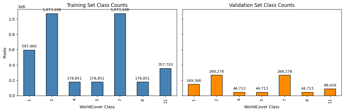
Raw class counts: {1: 746826, 2: 2360909, 4: 16934, 5: 135309, 7: 6155810, 8: 21538, 11: 447129} | CAP=1,341,387 FLOOR=223,564
X_train_cudf = cudf.DataFrame(X_train_cp, columns=band_names)
y_train_cudf = cudf.Series(y_train_cp, name="worldcover")
X_test_cudf = cudf.DataFrame(X_test_cp, columns=band_names)
y_test_cudf = cudf.Series(y_test_cp, name="worldcover")
6. Inspect Class Balance Before Training#
Plot the per-class pixel counts for the training and validation splits to confirm you carried enough samples forward for each label. Run this cell to visualize the distributions side by side with annotated totals.
Compare this against what the raw data looks like. Before rebalancing, the urban AOI alone left flooded vegetation, crops and bare ground with so little support that the model never predicted them at all. After adding the second AOI and applying the cap-and-floor rebalancing above, every class carries enough samples to be learnable, and the counts fall within a much narrower band. The remaining skew is intentional: we compress the imbalance rather than eliminate it, because the underlying landscape genuinely is mostly built area and trees.
train_counts = y_train_cudf.value_counts().sort_index().to_pandas()
test_counts = y_test_cudf.value_counts().sort_index().to_pandas()

fig, ax = plt.subplots(1, 2, figsize=(12, 4), sharey=True)
train_counts.plot(kind="bar", ax=ax[0], color="steelblue", edgecolor="black")
ax[0].set_title("Training Set Class Counts")
ax[0].set_xlabel("WorldCover Class")
ax[0].set_ylabel("Pixels")

test_counts.plot(kind="bar", ax=ax[1], color="darkorange", edgecolor="black")
ax[1].set_title("Validation Set Class Counts")
ax[1].set_xlabel("WorldCover Class")

# Annotate bars
for axis, counts in zip(ax, [train_counts, test_counts], strict=False):
    for patch, val in zip(axis.patches, counts.values, strict=False):
        axis.annotate(
            f"{int(val):,}",
            (patch.get_x() + patch.get_width() / 2, patch.get_height()),
            ha="center",
            va="bottom",
            fontsize=9,
            xytext=(0, 4),
            textcoords="offset points",
        )

plt.tight_layout()
plt.show()
7. Train a cuML Random Forest on the GPU#
Instantiate the cuML RandomForestClassifier and fit it on the cuDF training table. Run this cell to launch GPU-accelerated training; the estimator consumes the cuDF inputs directly and keeps the model resident on device for rapid evaluation in the following steps.
A few of the hyperparameters below are deliberate rather than default:
max_features=0.5considers three of our six features at each split. Thesqrtdefault works out to two features, which is stingy when the feature set is this small and the bands are correlated.min_samples_leaf=16prevents leaves from memorizing the oversampled rare-class rows, which appear multiple times after rebalancing.max_depth=16is cuML’s default, stated explicitly so the model is reproducible if that default ever changes.n_streams=1makes training deterministic givenrandom_state. Raise it to 4 for a speedup if you do not need bit-identical runs.
rf = RandomForestClassifier(
    n_estimators=300,
    n_bins=256,
    n_streams=1,  # deterministic with random_state; use 4 for speed if you don't care
    bootstrap=True,
    split_criterion="gini",
    max_features=0.5,  # 3 of 6 features per split (default sqrt≈2 is stingy here)
    min_samples_leaf=16,  # stops leaves from memorizing the 10-13x duplicated rare classes
    max_depth=16,  # cuML default, stated explicitly
    random_state=random_state,
)

rf.fit(X_train_cudf, y_train_cudf)
RandomForestClassifier()In a Jupyter environment, please rerun this cell to show the HTML representation or trust the notebook.
On GitHub, the HTML representation is unable to render, please try loading this page with nbviewer.org.
RandomForestClassifier()
While the model training is in progress, if you want to visualize the system hardware metrics and understand GPU and memory consumption within your Jupyterlab environment, consider using the NVDashboard Jupyterlab extension.
8. Score the Model and Build a Confusion Matrix#
Evaluate the trained forest on the validation split by predicting in GPU memory and computing accuracy with cuML. We report two numbers here, and the gap between them is the point.
Accuracy answers “what fraction of pixels did we get right?” - which a model can score well on simply by predicting the majority class everywhere. Macro-F1 averages the per-class F1 scores with equal weight, so a class the model never predicts drags it down no matter how rare that class is. Reporting only accuracy on land-cover data is how a model that ignores three of seven classes ends up looking respectable.
Run this cell to print both scores and produce an xarray.DataArray you can visualize in the next step.
pred_gpu = rf.predict(X_test_cudf)

val_acc = accuracy_score(y_test_cudf, pred_gpu)
print(f"Validation accuracy: {val_acc:.3f}")

pred_cpu = pred_gpu.to_pandas()
test_cpu = y_test_cudf.to_pandas()

# Macro-F1 weights every class equally, so it exposes rare-class performance
# that overall accuracy (dominated by Built Area) hides.
f1_macro = f1_score(test_cpu, pred_cpu, labels=valid_classes, average="macro")
print(f"Macro-F1 (equal weight per class): {f1_macro:.3f}")

cm = confusion_matrix(test_cpu, pred_cpu, labels=valid_classes)
cm_da = xr.DataArray(
    cm,
    coords={"actual": valid_classes, "predicted": valid_classes},
    dims=("actual", "predicted"),
)
cm_da
Validation accuracy: 0.781
Macro-F1 (equal weight per class): 0.729
<xarray.DataArray (actual: 7, predicted: 7)> Size: 392B
array([[132595,   3819,   5632,     28,   6806,    111,    375],
       [  1040, 240226,   1538,    171,  19571,      0,   5732],
       [   864,   4492,  25534,    119,  11007,      5,   2692],
       [    68,   2526,    152,  19940,  14008,      2,   8017],
       [  2419,  35187,   1648,   6076, 206903,   4382,  11663],
       [   140,     56,     20,    675,   5359,  38446,     17],
       [   605,  10815,   1552,   7159,  22425,      7,  46863]])
Coordinates:
  * actual     (actual) int64 56B 1 2 4 5 7 8 11
* predicted (predicted) int64 56B 1 2 4 5 7 8 119. Visualize Confusion Matrix and Interpret Class Coverage#
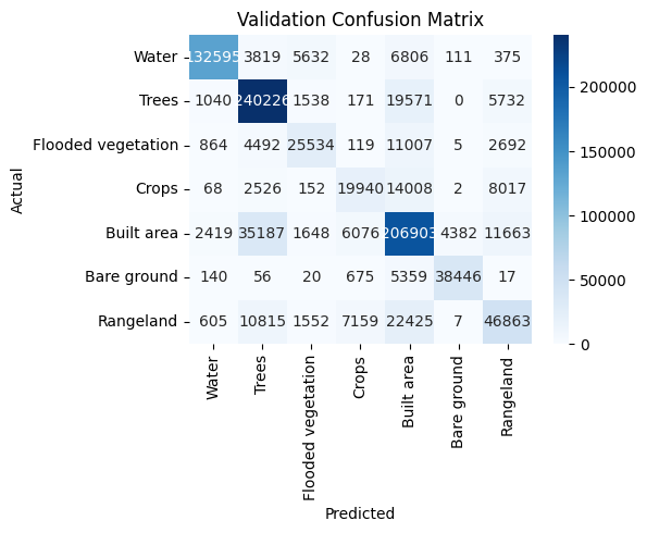
Plot the confusion matrix to see where the model succeeds and where it still struggles. Run this cell to render the heatmap.
Note
Adding the second AOI and rebalancing traded headline accuracy for balanced performance: accuracy fell from 0.908 to 0.781, while macro-F1 rose from roughly 0.3 to 0.729 and every class is now predicted. The earlier 0.908 was measuring the model’s ability to say “built area” in a mostly built-up scene.
cm = confusion_matrix(test_cpu, pred_cpu, labels=valid_classes)
labels_pretty = [worldcover_classes[c] for c in valid_classes]

plt.figure(figsize=(6, 5))
sns.heatmap(
    cm,
    annot=True,
    fmt="d",
    cmap="Blues",
    xticklabels=labels_pretty,
    yticklabels=labels_pretty,
)
plt.title("Validation Confusion Matrix")
plt.xlabel("Predicted")
plt.ylabel("Actual")
plt.tight_layout()
plt.show()
10. Review Precision/Recall by Class#
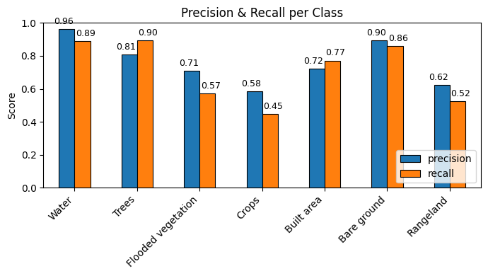
Summarize model performance with per-class precision and recall. Run this cell to chart the scores.
Every class now scores non-zero, but they do not score equally. Water (F1 0.92), bare ground (0.88) and trees (0.85) are separated cleanly by NDVI and NDWI. Built area (0.75) and flooded vegetation (0.63) are respectable. Crops (0.51) and rangeland (0.57) are the weak points, and the confusion matrix above shows why: both are frequently predicted as built area. An annual median flattens the growth cycle that distinguishes cropland from bare or developed ground, and the four visible/near-infrared bands we use cannot see the moisture difference that would separate them. Adding the SWIR bands B11 and B12 is the most promising next step, and we return to it at the end of the notebook.
report = classification_report(
    test_cpu,
    pred_cpu,
    labels=valid_classes,
    output_dict=True,
)
pr_table = pd.DataFrame(report).loc[["precision", "recall"], map(str, valid_classes)].T
pr_table.index = labels_pretty

ax = pr_table.plot(kind="bar", linewidth=0.8, edgecolor="black", figsize=(7, 4))
ax.set_title("Precision & Recall per Class")
ax.set_ylabel("Score")
ax.set_ylim(0, 1)
ax.set_xticklabels(labels_pretty, rotation=45, ha="right")
ax.legend(loc="lower right")

for i, container in enumerate(ax.containers):
    shift = -0.05 if i == 0 else 0.05  # adjust per container
    for patch, val in zip(container.patches, container.datavalues, strict=False):
        ax.annotate(
            f"{val:.2f}",
            (
                patch.get_x() + patch.get_width() / 2 + shift,
                patch.get_height(),
            ),
            ha="center",
            va="bottom",
            fontsize=9,
            xytext=(0, 3),
            textcoords="offset points",
        )

plt.tight_layout()
plt.show()
11. Persist the Trained Model#
Save the fitted Random Forest so you can reload it for inference. Run this cell to create the model directory if needed and pickle the cuML estimator. Keeping a serialized copy lets you deploy predictions without retraining or rerunning the feature pipeline.
with open(str(MODEL_PATH), "wb") as f:
    pickle.dump(rf, f)
Stage 3 · Run Inference and Publish the classification tile#
Now that we have finished training the model, in this stage we load the saved Random Forest model, pull a fresh Sentinel-2 tile, compute the familiar spectral features on the GPU, and classify each pixel. After reshaping the predictions into a raster, we compare them against the tile’s true-color composite to compare the two, then write the result to a Cloud-Optimized GeoTIFF (locally or to S3).
1. Reload the Trained Model#
Start by bringing the serialized Random Forest back into memory. Run this cell to unpickle the estimator you saved in Stage 2; the returned object keeps its GPU parameters and is ready to score new tiles without retraining.
with open(str(MODEL_PATH), "rb") as f:
    rf = pickle.load(f)
rf
RandomForestClassifier()In a Jupyter environment, please rerun this cell to show the HTML representation or trust the notebook.
On GitHub, the HTML representation is unable to render, please try loading this page with nbviewer.org.
RandomForestClassifier()
2. Locate the Sentinel-2 Tile to Score#
Connect to the Planetary Computer STAC endpoint, supply the Sentinel-2 tile ID you want to score, and stage the COG output path.
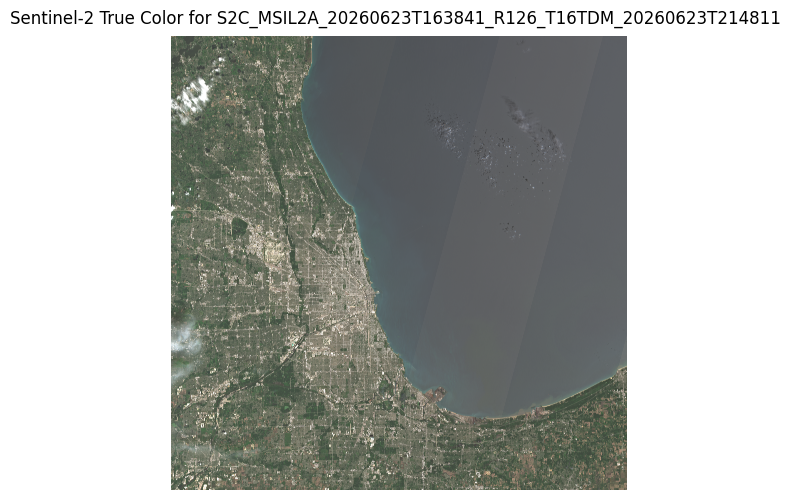
This example targets S2C_MSIL2A_20260623T163841_R126_T16TDM_20260623T214811, a tile over the Chicago metropolitan area in UTM zone 16 - a region the model has never seen, since training covered Minnesota and New York. Sentinel-2C scenes carry the same Level-2A product and band set as 2A and 2B, so no changes are needed to consume one.
An earlier revision scored a Manhattan tile, which turned out to be a poor demonstration: the long shadows cast by tall buildings push NDWI positive, and the model dutifully labelled downtown as water. It is a useful reminder that a spectral index is a proxy, not a measurement, and that dense urban cores are a genuinely hard case for a model trained on annual medians.
Run these cells to verify the tile exists and fetch its STAC item before you start feature extraction.
stac_client = Client.open(CATALOG_URL, modifier=planetary_computer.sign_inplace)

tile_id = "S2C_MSIL2A_20260623T163841_R126_T16TDM_20260623T214811"  # replace as needed
UPLOAD_TO_S3 = False
cog_path = INFERENCE_OUTPUT_DIR / f"lulc_{tile_id}.tif"
search = stac_client.search(
    collections=["sentinel-2-l2a"],
    ids=[tile_id],
)
items = list(search.items())
if not items:
    raise ValueError(f"No Sentinel-2 L2A items found for '{tile_id}'")

item = items[0]
item
3. Fetch and Stack the Target Tile#
Derive the tile’s EPSG code from the STAC metadata, then build a stackstac raster for the bands the model expects. Run this cell to fetch the single-scene cube at 10 m resolution with 2,048×2,048 chunks. Any missing metadata raises an error so you can choose another tile.
We fetch SCL alongside the four spectral bands here. Training data was cloud-masked, so inference must be too - scoring unmasked pixels would feed the model cloud tops and shadows it never saw during training, and it would confidently label them as something.
epsg_code = item.properties.get("proj:epsg")
if epsg_code is None:
    proj_code = item.properties.get("proj:code")
    if proj_code:
        epsg_code = int(proj_code.split(":")[-1])
    else:
        raise ValueError("No proj:epsg/proj:code in item")

# Fetch SCL alongside the spectral bands so we can mask clouds/shadows at
# inference time exactly as we did in training.
INFER_ASSETS = BANDS + ["SCL"]
stack = (
    stackstac.stack(
        [item],
        assets=INFER_ASSETS,
        resolution=10,
        epsg=epsg_code,
        fill_value=np.nan,
        chunksize=(1, 1, 2048, 2048),
        rescale=False,
        resampling=rasterio.enums.Resampling.nearest,  # keep SCL codes intact
    )
    .squeeze("time")
    .assign_coords(band=INFER_ASSETS)
    .astype("float32")
)

stack
<xarray.DataArray 'stackstac-1ff43b0298c5e2a1def6be96e51a8443' (band: 5,
                                                                y: 11120,
                                                                x: 11152)> Size: 2GB
dask.array<astype, shape=(5, 11120, 11152), dtype=float32, chunksize=(1, 2048, 2048), chunktype=numpy.ndarray>
Coordinates: (12/43)
  * band                                     (band) <U3 60B 'B02' ... 'SCL'
  * y                                        (y) float64 89kB 4.701e+06 ... 4...
  * x                                        (x) float64 89kB 3.984e+05 ... 5...
    time                                     datetime64[ns] 8B 2026-06-23T16:...
    id                                       <U54 216B 'S2C_MSIL2A_20260623T1...
    s2:cloud_shadow_percentage               float64 8B 0.0142
    ...                                       ...
    gsd                                      (band) float64 40B 10.0 ... 20.0
    title                                    (band) <U29 580B 'Band 2 - Blue ...
    common_name                              (band) object 40B 'blue' ... None
    center_wavelength                        (band) object 40B 0.49 ... None
    full_width_half_max                      (band) object 40B 0.098 ... None
    epsg                                     int64 8B 32616
Attributes:
    spec:        RasterSpec(epsg=32616, bounds=(398400, 4589550, 509920, 4700...
    crs:         epsg:32616
    transform:   | 10.00, 0.00, 398400.00|\n| 0.00,-10.00, 4700750.00|\n| 0.0...
resolution: 104. Inspect the Tile with a Quick True-Color Preview#
Render a stretched RGB composite so you can sanity-check the tile before running inference. Execute this cell to pull the red, green, and blue bands, normalized to a 99th-percentile stretch, and display a true-color image for the tile corresponding to the tile_id. Use the preview to confirm the scene is cloud-free and matches the area you expect. If not, pick a different Sentinel-2 tile ID before proceeding.
red_np = stack.sel(band="B04").data.compute().astype(np.float32)
green_np = stack.sel(band="B03").data.compute().astype(np.float32)
blue_np = stack.sel(band="B02").data.compute().astype(np.float32)

rgb_np = np.stack([red_np, green_np, blue_np], axis=0)
stretch = np.nanpercentile(rgb_np, 99)
rgb_np = np.clip(rgb_np / stretch, 0, 1)
rgb_img = np.moveaxis(rgb_np, 0, -1)

plt.figure(figsize=(6, 6))
plt.imshow(rgb_img)
plt.title(f"Sentinel-2 True Color for {tile_id}")
plt.axis("off")
plt.show()
5. Engineer Features on the GPU and Run Inference#
Compute the same band stack, NDVI, and NDWI features the model saw during training, apply the clear-sky mask, and flatten the result to per-pixel rows before prediction. Run these cells to convert the Sentinel tile into a cuDF table, call rf.predict, and inspect the label counts.
The band values are pulled in a single .compute() rather than one call per band, which avoids re-reading the same chunks from the remote store four times over.
# Clear-sky mask from SCL (same classes used in training).
scl = cp.asarray(stack.sel(band="SCL").data.compute())
clear = cp.isin(scl, cp.asarray([4, 5, 6, 11]))

# One compute pulls all four spectral bands together instead of four round-trips.
bands_arr = cp.asarray(stack.sel(band=BANDS).data.compute())  # (4, y, x)
b02, b03, b04, b08 = bands_arr

ndvi = (b08 - b04) / (b08 + b04)
ndwi = (b03 - b08) / (b03 + b08)

y_coords = stack.y.values
x_coords = stack.x.values

feature_stack = cp.stack([b02, b03, b04, b08, ndvi, ndwi], axis=0)
flat = feature_stack.reshape(len(ALL_FEATURES), -1).T
mask = cp.isfinite(flat).all(axis=1) & clear.reshape(-1)

flat_valid = flat[mask]
features_df = cudf.DataFrame(flat_valid, columns=ALL_FEATURES)
preds = rf.predict(features_df)
preds
0             7
1            11
2            11
3            11
4            11
             ..
114945147     7
114945148     7
114945149     7
114945150     7
114945151     7
Length: 114945152, dtype: int32
preds.value_counts()
1     59061516
7     24168699
2     15236069
11    11933657
8      1831939
4      1567424
5      1145848
Name: count, dtype: int64
6. Reshape Predictions Back to the Tile Grid#
Restore the flat predictions to their native image layout so you can visualize and export them. This cell fills a nodata-initialized array, drops the predictions into the valid-pixel slots, reshapes everything to the tile’s y×x grid, and wraps the result in an xarray.DataArray with coordinates and metadata (tile ID, model name, acquisition datetime). Upon running it, the returned pred_da matches the raster geometry needed for plotting and COG creation.
full = cp.full(mask.shape[0], NODATA_VALUE, dtype=cp.int8)
full[mask] = preds.astype(cp.int8)

h, w = len(y_coords), len(x_coords)
grid = full.reshape(h, w)

pred_da = xr.DataArray(
    cp.asnumpy(grid),
    coords={"y": y_coords, "x": x_coords},
    dims=("y", "x"),
    name="worldcover_prediction",
).where(cp.asnumpy(mask.reshape(h, w)))

pred_da.attrs.update(
    {
        "tile_id": item.id,
        "model": MODEL_PATH.name,
        "datetime": item.properties["datetime"],
    }
)
pred_da
<xarray.DataArray 'worldcover_prediction' (y: 11120, x: 11152)> Size: 496MB
array([[nan, nan, nan, ..., nan, nan, nan],
       [nan, nan, nan, ..., nan, nan, nan],
       [nan, nan, nan, ..., nan, nan, nan],
       ...,
       [nan, nan, nan, ..., nan, nan, nan],
       [nan, nan, nan, ..., nan, nan, nan],
       [nan, nan, nan, ..., nan, nan, nan]],
      shape=(11120, 11152), dtype=float32)
Coordinates:
  * y        (y) float64 89kB 4.701e+06 4.701e+06 ... 4.59e+06 4.59e+06
  * x        (x) float64 89kB 3.984e+05 3.984e+05 ... 5.099e+05 5.099e+05
Attributes:
    tile_id:   S2C_MSIL2A_20260623T163841_R126_T16TDM_20260623T214811
    model:     lulc_rf_2022.pkl
datetime: 2026-06-23T16:38:41.025000Z7. Compare the True-Color Tile with Model Predictions#
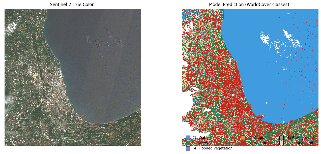
Plot the Sentinel-2 RGB composite alongside the inferred land-cover map to sanity-check the output. Run this cell to render both views with matching coordinates and a legend keyed to the WorldCover classes.
Read the two panels together. Lake Michigan and the river corridors come through cleanly as water, the parks and the agricultural land west of the city separate from the urban core, and the built-up grid is recognisable as such. The boundaries between crops and rangeland on the western edge are the least convincing part of the map, consistent with the per-class scores in Stage 2. Areas masked out as cloud or shadow carry the nodata value and appear as gaps.
# Build an RGB DataArray using the tile’s coordinates
rgb_da = xr.DataArray(
    rgb_img,
    dims=("y", "x", "band"),
    coords={"y": stack.y.values, "x": stack.x.values, "band": ["R", "G", "B"]},
)

worldcover_colors = {
    1: "#419bdf",
    2: "#397d49",
    4: "#7a87c6",
    5: "#e49635",
    7: "#c4281b",
    8: "#a59b8f",
    11: "#e3e2c3",
}
classes = list(worldcover_colors.keys())
cmap = ListedColormap([worldcover_colors[i] for i in classes])
norm = BoundaryNorm(classes + [classes[-1] + 1], cmap.N)

fig, axes = plt.subplots(1, 2, figsize=(14, 6), constrained_layout=True)

# Left: true-color tile (coordinates from stack)
rgb_da.plot.imshow(
    ax=axes[0],
    rgb="band",
    add_colorbar=False,
)
axes[0].set_title("Sentinel-2 True Color")
axes[0].set_aspect("equal")
axes[0].axis("off")

# Right: predicted classes
pred_da.plot.imshow(
    ax=axes[1],
    cmap=cmap,
    norm=norm,
    add_colorbar=False,
)
axes[1].set_title("Model Prediction (WorldCover classes)")
axes[1].set_aspect("equal")
axes[1].axis("off")

legend_handles = [
    plt.Line2D(
        [0],
        [0],
        marker="s",
        color="none",
        markerfacecolor=worldcover_colors[c],
        markersize=12,
        linestyle="",
        label=f"{c}: {worldcover_classes[c]}",
    )
    for c in classes
]
axes[1].legend(
    handles=legend_handles,
    loc="lower center",
    bbox_to_anchor=(0.5, -0.05),
    ncol=3,
    frameon=False,
)

plt.show()
8. Export Predictions as a Cloud-Optimized GeoTIFF#
Write the labeled raster to disk so you can share or publish the map. This cell stamps CRS, transform and nodata metadata on pred_da, writes a temporary GeoTIFF, and uses cog_translate to produce the final COG either locally or directly to S3 (toggle UPLOAD_TO_S3 as needed). Run it to generate the lulc_<tile_id>.tif output; the temporary file is removed automatically when saving locally.
The output is written as int8. WorldCover class codes run from 1 to 11 and nodata is 0, so a signed byte is ample and halves the file size against int16. Tagging the nodata value explicitly means GIS software will render masked pixels as transparent rather than as a spurious class.
INFERENCE_OUTPUT_DIR.mkdir(parents=True, exist_ok=True)
temp_tif = cog_path.with_suffix(".tmp.tif")

pred_da.rio.write_crs(stack.rio.crs, inplace=True)
pred_da.rio.write_transform(stack.rio.transform(), inplace=True)
pred_da.rio.write_nodata(NODATA_VALUE, inplace=True)
# Class codes are 1-11, so int8 halves the on-disk/memory footprint vs int16.
pred_da.fillna(NODATA_VALUE).rio.to_raster(temp_tif, dtype="int8")

if UPLOAD_TO_S3:
    s3_vsis = f"/vsis3/{S3_BUCKET}/{S3_PREFIX.rstrip('/')}/{cog_path.name}"
    cog_translate(temp_tif, s3_vsis, COG_PROFILE, in_memory=False, quiet=False)
else:
    cog_translate(temp_tif, cog_path, COG_PROFILE, in_memory=False, quiet=False)
    temp_tif.unlink(missing_ok=True)
    print("Saved COG:", cog_path)
Summary#
We have built an end-to-end ML workflow on Sentinel-2 and ESA WorldCover imagery, from acquisition through to a land-cover classification map over an unseen tile. Along the way we touched a good part of the RAPIDS ecosystem: streaming scenes with Dask, cleaning and compositing them with Dask-backed Xarray, moving the samples on device with cupy-xarray, training a cuML random forest, and generating predictions into a Cloud-Optimized GeoTIFF.
It is worth being clear about where the acceleration actually came from. Training and inference are compute-bound and run entirely on the GPU, and that is where the speedup lives. Stage 1 is dominated by streaming tens of gigabytes of imagery over the network, so its runtime is governed by I/O rather than by arithmetic and Dask’s parallelism is what helps there.
Future Steps#
The class imbalance that was in the prior version of this notebook has been addressed, but the model still has a clear weak spot: crops (F1 0.51) and rangeland (0.57), both frequently confused with built area. Three directions are worth pursuing.
Add the SWIR bands. B11 and B12 sit at 1.6 µm and 2.2 µm and respond to vegetation moisture and soil composition in ways that the visible and near-infrared bands cannot. They are the single most likely fix for the crops/rangeland confusion. They arrive at 20 m and would need resampling to the 10 m grid, and adding them means re-running Stage 1.
Move beyond an annual median. Collapsing a year to one value discards phenology which is the seasonal growth cycle that most clearly separates cropland from permanent cover. Seasonal composites, or simple per-pixel statistics like the standard deviation across the year, would give the model something to work with.
Broaden the training footprint. Two AOIs is enough to demonstrate the problem and the fix, but a model intended for real use would want AOIs spanning more climate zones and more of the rare classes.
One operational improvement is also worth noting: Stage 1 currently holds every AOI’s stack in memory at once. Processing AOIs sequentially and releasing each stack after its Zarr write would roughly halve peak memory for the two-AOI case, and makes the notebook runnable on considerably smaller machines.