Perform Time Series Forecasting on Google Kubernetes Engine with NVIDIA GPUs#
October, 2023
In this example, we will be looking at a real-world example of time series forecasting with data from the M5 Forecasting Competition. Walmart provides historical sales data from multiple stores in three states, and our job is to predict the sales in a future 28-day period.
Prerequisites#
Prepare GKE cluster#
To run the example, you will need a working Google Kubernetes Engine (GKE) cluster with access to NVIDIA GPUs.
See Documentation
Set up a Google Kubernetes Engine (GKE) cluster with access to NVIDIA GPUs. Follow instructions in Google Kubernetes Engine.
To ensure that the example runs smoothly, ensure that you have ample memory in your GPUs. This notebook has been tested with NVIDIA A100.
Set up Dask-Kubernetes integration by following instructions in the following guides:
Kubeflow is not strictly necessary, but we highly recommend it, as Kubeflow gives you a nice notebook environment to run this notebook within the k8s cluster. (You may choose any method; we tested this example after installing Kubeflow from manifests.) When creating the notebook environment, use the following configuration:
2 CPUs, 16 GiB of memory
1 NVIDIA GPU
40 GiB disk volume
After uploading all the notebooks in the example, run this notebook (notebook.ipynb) in the notebook environment.
Note: We will use the worker pods to speed up the training stage. The preprocessing steps will run solely on the scheduler node.
Prepare a bucket in Google Cloud Storage#
Create a new bucket in Google Cloud Storage. Make sure that the worker pods in the k8s cluster has read/write access to this bucket. This can be done in one of the following methods:
Option 1: Specify an additional scope when provisioning the GKE cluster.
When you are provisioning a new GKE cluster, add the
storage-rwscope. This option is only available if you are creating a new cluster from scratch. If you are using an existing GKE cluster, see Option 2.Example:
gcloud container clusters create my_new_cluster --accelerator type=nvidia-tesla-t4 \
   --machine-type n1-standard-32 --zone us-central1-c --release-channel stable \
   --num-nodes 5 --scopes=gke-default,storage-rw
Option 2: Grant bucket access to the associated service account.
Find out which service account is associated with your GKE cluster. You can grant the bucket access to the service account as follows: Navigate to the Cloud Storage console, open the Bucket Details page for the bucket, open the Permissions tab, and click on Grant Access.
Enter the name of the bucket that your cluster has read-write access to:
bucket_name = "<Put the name of the bucket here>"
Install Python packages in the notebook environment#
!pip install kaggle gcsfs dask-kubernetes optuna
# Test if the bucket is accessible
import gcsfs

fs = gcsfs.GCSFileSystem()
fs.ls(f"{bucket_name}/")
[]
Obtain the time series data set from Kaggle#
If you do not yet have an account with Kaggle, create one now. Then follow instructions in Public API Documentation of Kaggle to obtain the API key. This step is needed to obtain the training data from the M5 Forecasting Competition. Once you obtained the API key, fill in the following:
kaggle_username = "<Put your Kaggle username here>"
kaggle_api_key = "<Put your Kaggle API key here>"
Now we are ready to download the data set:
%env KAGGLE_USERNAME=$kaggle_username
%env KAGGLE_KEY=$kaggle_api_key

!kaggle competitions download -c m5-forecasting-accuracy
Let’s unzip the ZIP archive and see what’s inside.
import zipfile

with zipfile.ZipFile("m5-forecasting-accuracy.zip", "r") as zf:
    zf.extractall(path="./data")
!ls -lh data/*.csv
-rw-r--r-- 1 rapids conda 102K Sep 28 18:59 data/calendar.csv
-rw-r--r-- 1 rapids conda 117M Sep 28 18:59 data/sales_train_evaluation.csv
-rw-r--r-- 1 rapids conda 115M Sep 28 18:59 data/sales_train_validation.csv
-rw-r--r-- 1 rapids conda 5.0M Sep 28 18:59 data/sample_submission.csv
-rw-r--r-- 1 rapids conda 194M Sep 28 18:59 data/sell_prices.csv
Data Preprocessing#
We are now ready to run the preprocessing steps.
Import modules and define utility functions#
import gc
import pathlib

import cudf
import gcsfs
import numpy as np


def sizeof_fmt(num, suffix="B"):
    for unit in ["", "Ki", "Mi", "Gi", "Ti", "Pi", "Ei", "Zi"]:
        if abs(num) < 1024.0:
            return f"{num:3.1f}{unit}{suffix}"
        num /= 1024.0
    return f"{num:.1f}Yi{suffix}"


def report_dataframe_size(df, name):
    mem_usage = sizeof_fmt(grid_df.memory_usage(index=True).sum())
    print(f"{name} takes up {mem_usage} memory on GPU")
Load Data#
TARGET = "sales"  # Our main target
END_TRAIN = 1941  # Last day in train set
raw_data_dir = pathlib.Path("./data/")
train_df = cudf.read_csv(raw_data_dir / "sales_train_evaluation.csv")
prices_df = cudf.read_csv(raw_data_dir / "sell_prices.csv")
calendar_df = cudf.read_csv(raw_data_dir / "calendar.csv").rename(
    columns={"d": "day_id"}
)
train_df
| id | item_id | dept_id | cat_id | store_id | state_id | d_1 | d_2 | d_3 | d_4 | ... | d_1932 | d_1933 | d_1934 | d_1935 | d_1936 | d_1937 | d_1938 | d_1939 | d_1940 | d_1941 | |
|---|---|---|---|---|---|---|---|---|---|---|---|---|---|---|---|---|---|---|---|---|---|
| 0 | HOBBIES_1_001_CA_1_evaluation | HOBBIES_1_001 | HOBBIES_1 | HOBBIES | CA_1 | CA | 0 | 0 | 0 | 0 | ... | 2 | 4 | 0 | 0 | 0 | 0 | 3 | 3 | 0 | 1 |
| 1 | HOBBIES_1_002_CA_1_evaluation | HOBBIES_1_002 | HOBBIES_1 | HOBBIES | CA_1 | CA | 0 | 0 | 0 | 0 | ... | 0 | 1 | 2 | 1 | 1 | 0 | 0 | 0 | 0 | 0 |
| 2 | HOBBIES_1_003_CA_1_evaluation | HOBBIES_1_003 | HOBBIES_1 | HOBBIES | CA_1 | CA | 0 | 0 | 0 | 0 | ... | 1 | 0 | 2 | 0 | 0 | 0 | 2 | 3 | 0 | 1 |
| 3 | HOBBIES_1_004_CA_1_evaluation | HOBBIES_1_004 | HOBBIES_1 | HOBBIES | CA_1 | CA | 0 | 0 | 0 | 0 | ... | 1 | 1 | 0 | 4 | 0 | 1 | 3 | 0 | 2 | 6 |
| 4 | HOBBIES_1_005_CA_1_evaluation | HOBBIES_1_005 | HOBBIES_1 | HOBBIES | CA_1 | CA | 0 | 0 | 0 | 0 | ... | 0 | 0 | 0 | 2 | 1 | 0 | 0 | 2 | 1 | 0 |
| ... | ... | ... | ... | ... | ... | ... | ... | ... | ... | ... | ... | ... | ... | ... | ... | ... | ... | ... | ... | ... | ... |
| 30485 | FOODS_3_823_WI_3_evaluation | FOODS_3_823 | FOODS_3 | FOODS | WI_3 | WI | 0 | 0 | 2 | 2 | ... | 1 | 0 | 3 | 0 | 1 | 1 | 0 | 0 | 1 | 1 |
| 30486 | FOODS_3_824_WI_3_evaluation | FOODS_3_824 | FOODS_3 | FOODS | WI_3 | WI | 0 | 0 | 0 | 0 | ... | 0 | 0 | 0 | 0 | 0 | 0 | 1 | 0 | 1 | 0 |
| 30487 | FOODS_3_825_WI_3_evaluation | FOODS_3_825 | FOODS_3 | FOODS | WI_3 | WI | 0 | 6 | 0 | 2 | ... | 0 | 0 | 1 | 2 | 0 | 1 | 0 | 1 | 0 | 2 |
| 30488 | FOODS_3_826_WI_3_evaluation | FOODS_3_826 | FOODS_3 | FOODS | WI_3 | WI | 0 | 0 | 0 | 0 | ... | 1 | 1 | 1 | 4 | 6 | 0 | 1 | 1 | 1 | 0 |
| 30489 | FOODS_3_827_WI_3_evaluation | FOODS_3_827 | FOODS_3 | FOODS | WI_3 | WI | 0 | 0 | 0 | 0 | ... | 1 | 2 | 0 | 5 | 4 | 0 | 2 | 2 | 5 | 1 |
30490 rows × 1947 columns
The columns d_1, d_2, …, d_1941 indicate the sales data at days 1, 2, …, 1941 from 2011-01-29.
prices_df
| store_id | item_id | wm_yr_wk | sell_price | |
|---|---|---|---|---|
| 0 | CA_1 | HOBBIES_1_001 | 11325 | 9.58 |
| 1 | CA_1 | HOBBIES_1_001 | 11326 | 9.58 |
| 2 | CA_1 | HOBBIES_1_001 | 11327 | 8.26 |
| 3 | CA_1 | HOBBIES_1_001 | 11328 | 8.26 |
| 4 | CA_1 | HOBBIES_1_001 | 11329 | 8.26 |
| ... | ... | ... | ... | ... |
| 6841116 | WI_3 | FOODS_3_827 | 11617 | 1.00 |
| 6841117 | WI_3 | FOODS_3_827 | 11618 | 1.00 |
| 6841118 | WI_3 | FOODS_3_827 | 11619 | 1.00 |
| 6841119 | WI_3 | FOODS_3_827 | 11620 | 1.00 |
| 6841120 | WI_3 | FOODS_3_827 | 11621 | 1.00 |
6841121 rows × 4 columns
calendar_df
| date | wm_yr_wk | weekday | wday | month | year | day_id | event_name_1 | event_type_1 | event_name_2 | event_type_2 | snap_CA | snap_TX | snap_WI | |
|---|---|---|---|---|---|---|---|---|---|---|---|---|---|---|
| 0 | 2011-01-29 | 11101 | Saturday | 1 | 1 | 2011 | d_1 | <NA> | <NA> | <NA> | <NA> | 0 | 0 | 0 |
| 1 | 2011-01-30 | 11101 | Sunday | 2 | 1 | 2011 | d_2 | <NA> | <NA> | <NA> | <NA> | 0 | 0 | 0 |
| 2 | 2011-01-31 | 11101 | Monday | 3 | 1 | 2011 | d_3 | <NA> | <NA> | <NA> | <NA> | 0 | 0 | 0 |
| 3 | 2011-02-01 | 11101 | Tuesday | 4 | 2 | 2011 | d_4 | <NA> | <NA> | <NA> | <NA> | 1 | 1 | 0 |
| 4 | 2011-02-02 | 11101 | Wednesday | 5 | 2 | 2011 | d_5 | <NA> | <NA> | <NA> | <NA> | 1 | 0 | 1 |
| ... | ... | ... | ... | ... | ... | ... | ... | ... | ... | ... | ... | ... | ... | ... |
| 1964 | 2016-06-15 | 11620 | Wednesday | 5 | 6 | 2016 | d_1965 | <NA> | <NA> | <NA> | <NA> | 0 | 1 | 1 |
| 1965 | 2016-06-16 | 11620 | Thursday | 6 | 6 | 2016 | d_1966 | <NA> | <NA> | <NA> | <NA> | 0 | 0 | 0 |
| 1966 | 2016-06-17 | 11620 | Friday | 7 | 6 | 2016 | d_1967 | <NA> | <NA> | <NA> | <NA> | 0 | 0 | 0 |
| 1967 | 2016-06-18 | 11621 | Saturday | 1 | 6 | 2016 | d_1968 | <NA> | <NA> | <NA> | <NA> | 0 | 0 | 0 |
| 1968 | 2016-06-19 | 11621 | Sunday | 2 | 6 | 2016 | d_1969 | NBAFinalsEnd | Sporting | Father's day | Cultural | 0 | 0 | 0 |
1969 rows × 14 columns
Reformat sales times series data#
Pivot the columns d_1, d_2, …, d_1941 into separate rows using cudf.melt.
index_columns = ["id", "item_id", "dept_id", "cat_id", "store_id", "state_id"]
grid_df = cudf.melt(
    train_df, id_vars=index_columns, var_name="day_id", value_name=TARGET
)
grid_df
| id | item_id | dept_id | cat_id | store_id | state_id | day_id | sales | |
|---|---|---|---|---|---|---|---|---|
| 0 | HOBBIES_1_001_CA_1_evaluation | HOBBIES_1_001 | HOBBIES_1 | HOBBIES | CA_1 | CA | d_1 | 0 |
| 1 | HOBBIES_1_002_CA_1_evaluation | HOBBIES_1_002 | HOBBIES_1 | HOBBIES | CA_1 | CA | d_1 | 0 |
| 2 | HOBBIES_1_003_CA_1_evaluation | HOBBIES_1_003 | HOBBIES_1 | HOBBIES | CA_1 | CA | d_1 | 0 |
| 3 | HOBBIES_1_004_CA_1_evaluation | HOBBIES_1_004 | HOBBIES_1 | HOBBIES | CA_1 | CA | d_1 | 0 |
| 4 | HOBBIES_1_005_CA_1_evaluation | HOBBIES_1_005 | HOBBIES_1 | HOBBIES | CA_1 | CA | d_1 | 0 |
| ... | ... | ... | ... | ... | ... | ... | ... | ... |
| 59181085 | FOODS_3_823_WI_3_evaluation | FOODS_3_823 | FOODS_3 | FOODS | WI_3 | WI | d_1941 | 1 |
| 59181086 | FOODS_3_824_WI_3_evaluation | FOODS_3_824 | FOODS_3 | FOODS | WI_3 | WI | d_1941 | 0 |
| 59181087 | FOODS_3_825_WI_3_evaluation | FOODS_3_825 | FOODS_3 | FOODS | WI_3 | WI | d_1941 | 2 |
| 59181088 | FOODS_3_826_WI_3_evaluation | FOODS_3_826 | FOODS_3 | FOODS | WI_3 | WI | d_1941 | 0 |
| 59181089 | FOODS_3_827_WI_3_evaluation | FOODS_3_827 | FOODS_3 | FOODS | WI_3 | WI | d_1941 | 1 |
59181090 rows × 8 columns
For each time series, add 28 rows that corresponds to the future forecast horizon:
add_grid = cudf.DataFrame()
for i in range(1, 29):
    temp_df = train_df[index_columns]
    temp_df = temp_df.drop_duplicates()
    temp_df["day_id"] = "d_" + str(END_TRAIN + i)
    temp_df[TARGET] = np.nan  # Sales amount at time (n + i) is unknown
    add_grid = cudf.concat([add_grid, temp_df])
add_grid["day_id"] = add_grid["day_id"].astype(
    "category"
)  # The day_id column is categorical, after cudf.melt

grid_df = cudf.concat([grid_df, add_grid])
grid_df = grid_df.reset_index(drop=True)
grid_df["sales"] = grid_df["sales"].astype(
    np.float32
)  # Use float32 type for sales column, to conserve memory
grid_df
| id | item_id | dept_id | cat_id | store_id | state_id | day_id | sales | |
|---|---|---|---|---|---|---|---|---|
| 0 | HOBBIES_1_001_CA_1_evaluation | HOBBIES_1_001 | HOBBIES_1 | HOBBIES | CA_1 | CA | d_1 | 0.0 |
| 1 | HOBBIES_1_002_CA_1_evaluation | HOBBIES_1_002 | HOBBIES_1 | HOBBIES | CA_1 | CA | d_1 | 0.0 |
| 2 | HOBBIES_1_003_CA_1_evaluation | HOBBIES_1_003 | HOBBIES_1 | HOBBIES | CA_1 | CA | d_1 | 0.0 |
| 3 | HOBBIES_1_004_CA_1_evaluation | HOBBIES_1_004 | HOBBIES_1 | HOBBIES | CA_1 | CA | d_1 | 0.0 |
| 4 | HOBBIES_1_005_CA_1_evaluation | HOBBIES_1_005 | HOBBIES_1 | HOBBIES | CA_1 | CA | d_1 | 0.0 |
| ... | ... | ... | ... | ... | ... | ... | ... | ... |
| 60034805 | FOODS_3_823_WI_3_evaluation | FOODS_3_823 | FOODS_3 | FOODS | WI_3 | WI | d_1969 | NaN |
| 60034806 | FOODS_3_824_WI_3_evaluation | FOODS_3_824 | FOODS_3 | FOODS | WI_3 | WI | d_1969 | NaN |
| 60034807 | FOODS_3_825_WI_3_evaluation | FOODS_3_825 | FOODS_3 | FOODS | WI_3 | WI | d_1969 | NaN |
| 60034808 | FOODS_3_826_WI_3_evaluation | FOODS_3_826 | FOODS_3 | FOODS | WI_3 | WI | d_1969 | NaN |
| 60034809 | FOODS_3_827_WI_3_evaluation | FOODS_3_827 | FOODS_3 | FOODS | WI_3 | WI | d_1969 | NaN |
60034810 rows × 8 columns
Free up GPU memory#
GPU memory is a precious resource, so let’s try to free up some memory. First, delete temporary variables we no longer need:
# Use xdel magic to scrub extra references from Jupyter notebook
%xdel temp_df
%xdel add_grid
%xdel train_df

# Invoke the garbage collector explicitly to free up memory
gc.collect()
8136
Second, let’s reduce the footprint of grid_df by converting strings into categoricals:
report_dataframe_size(grid_df, "grid_df")
grid_df takes up 5.2GiB memory on GPU
grid_df.dtypes
id            object
item_id       object
dept_id       object
cat_id        object
store_id      object
state_id      object
day_id      category
sales        float32
dtype: object
for col in index_columns:
    grid_df[col] = grid_df[col].astype("category")
    gc.collect()
report_dataframe_size(grid_df, "grid_df")
grid_df takes up 802.6MiB memory on GPU
grid_df.dtypes
id          category
item_id     category
dept_id     category
cat_id      category
store_id    category
state_id    category
day_id      category
sales        float32
dtype: object
Identify the release week of each product#
Each row in the prices_df table contains the price of a product sold at a store for a given week.
prices_df
| store_id | item_id | wm_yr_wk | sell_price | |
|---|---|---|---|---|
| 0 | CA_1 | HOBBIES_1_001 | 11325 | 9.58 |
| 1 | CA_1 | HOBBIES_1_001 | 11326 | 9.58 |
| 2 | CA_1 | HOBBIES_1_001 | 11327 | 8.26 |
| 3 | CA_1 | HOBBIES_1_001 | 11328 | 8.26 |
| 4 | CA_1 | HOBBIES_1_001 | 11329 | 8.26 |
| ... | ... | ... | ... | ... |
| 6841116 | WI_3 | FOODS_3_827 | 11617 | 1.00 |
| 6841117 | WI_3 | FOODS_3_827 | 11618 | 1.00 |
| 6841118 | WI_3 | FOODS_3_827 | 11619 | 1.00 |
| 6841119 | WI_3 | FOODS_3_827 | 11620 | 1.00 |
| 6841120 | WI_3 | FOODS_3_827 | 11621 | 1.00 |
6841121 rows × 4 columns
Notice that not all products were sold over every week. Some products were sold only during some weeks. Let’s use the groupby operation to identify the first week in which each product went on the shelf.
release_df = (
    prices_df.groupby(["store_id", "item_id"])["wm_yr_wk"].agg("min").reset_index()
)
release_df.columns = ["store_id", "item_id", "release_week"]
release_df
| store_id | item_id | release_week | |
|---|---|---|---|
| 0 | CA_4 | FOODS_3_529 | 11421 |
| 1 | TX_1 | HOUSEHOLD_1_409 | 11230 |
| 2 | WI_2 | FOODS_3_145 | 11214 |
| 3 | CA_4 | HOUSEHOLD_1_494 | 11106 |
| 4 | WI_3 | HOBBIES_1_093 | 11223 |
| ... | ... | ... | ... |
| 30485 | CA_3 | HOUSEHOLD_1_369 | 11205 |
| 30486 | CA_2 | FOODS_3_109 | 11101 |
| 30487 | CA_4 | FOODS_2_119 | 11101 |
| 30488 | CA_4 | HOUSEHOLD_2_384 | 11110 |
| 30489 | WI_3 | HOBBIES_1_135 | 11328 |
30490 rows × 3 columns
Now that we’ve computed the release week for each product, let’s merge it back to grid_df:
grid_df = grid_df.merge(release_df, on=["store_id", "item_id"], how="left")
grid_df = grid_df.sort_values(index_columns + ["day_id"]).reset_index(drop=True)
grid_df
| id | item_id | dept_id | cat_id | store_id | state_id | day_id | sales | release_week | |
|---|---|---|---|---|---|---|---|---|---|
| 0 | FOODS_1_001_CA_1_evaluation | FOODS_1_001 | FOODS_1 | FOODS | CA_1 | CA | d_1 | 3.0 | 11101 |
| 1 | FOODS_1_001_CA_1_evaluation | FOODS_1_001 | FOODS_1 | FOODS | CA_1 | CA | d_2 | 0.0 | 11101 |
| 2 | FOODS_1_001_CA_1_evaluation | FOODS_1_001 | FOODS_1 | FOODS | CA_1 | CA | d_3 | 0.0 | 11101 |
| 3 | FOODS_1_001_CA_1_evaluation | FOODS_1_001 | FOODS_1 | FOODS | CA_1 | CA | d_4 | 1.0 | 11101 |
| 4 | FOODS_1_001_CA_1_evaluation | FOODS_1_001 | FOODS_1 | FOODS | CA_1 | CA | d_5 | 4.0 | 11101 |
| ... | ... | ... | ... | ... | ... | ... | ... | ... | ... |
| 60034805 | HOUSEHOLD_2_516_WI_3_evaluation | HOUSEHOLD_2_516 | HOUSEHOLD_2 | HOUSEHOLD | WI_3 | WI | d_1965 | NaN | 11101 |
| 60034806 | HOUSEHOLD_2_516_WI_3_evaluation | HOUSEHOLD_2_516 | HOUSEHOLD_2 | HOUSEHOLD | WI_3 | WI | d_1966 | NaN | 11101 |
| 60034807 | HOUSEHOLD_2_516_WI_3_evaluation | HOUSEHOLD_2_516 | HOUSEHOLD_2 | HOUSEHOLD | WI_3 | WI | d_1967 | NaN | 11101 |
| 60034808 | HOUSEHOLD_2_516_WI_3_evaluation | HOUSEHOLD_2_516 | HOUSEHOLD_2 | HOUSEHOLD | WI_3 | WI | d_1968 | NaN | 11101 |
| 60034809 | HOUSEHOLD_2_516_WI_3_evaluation | HOUSEHOLD_2_516 | HOUSEHOLD_2 | HOUSEHOLD | WI_3 | WI | d_1969 | NaN | 11101 |
60034810 rows × 9 columns
del release_df  # No longer needed
gc.collect()
139
report_dataframe_size(grid_df, "grid_df")
grid_df takes up 1.2GiB memory on GPU
Filter out entries with zero sales#
We can further save space by dropping rows from grid_df that correspond to zero sales. Since each product doesn’t go on the shelf until its release week, its sale must be zero during any week that’s prior to the release week.
To make use of this insight, we bring in the wm_yr_wk column from calendar_df:
grid_df = grid_df.merge(calendar_df[["wm_yr_wk", "day_id"]], on=["day_id"], how="left")
grid_df
| id | item_id | dept_id | cat_id | store_id | state_id | day_id | sales | release_week | wm_yr_wk | |
|---|---|---|---|---|---|---|---|---|---|---|
| 0 | FOODS_1_001_WI_2_evaluation | FOODS_1_001 | FOODS_1 | FOODS | WI_2 | WI | d_809 | 0.0 | 11101 | 11312 |
| 1 | FOODS_1_001_WI_2_evaluation | FOODS_1_001 | FOODS_1 | FOODS | WI_2 | WI | d_810 | 0.0 | 11101 | 11312 |
| 2 | FOODS_1_001_WI_2_evaluation | FOODS_1_001 | FOODS_1 | FOODS | WI_2 | WI | d_811 | 2.0 | 11101 | 11312 |
| 3 | FOODS_1_001_WI_2_evaluation | FOODS_1_001 | FOODS_1 | FOODS | WI_2 | WI | d_812 | 0.0 | 11101 | 11312 |
| 4 | FOODS_1_001_WI_2_evaluation | FOODS_1_001 | FOODS_1 | FOODS | WI_2 | WI | d_813 | 1.0 | 11101 | 11313 |
| ... | ... | ... | ... | ... | ... | ... | ... | ... | ... | ... |
| 60034805 | HOUSEHOLD_2_516_WI_3_evaluation | HOUSEHOLD_2_516 | HOUSEHOLD_2 | HOUSEHOLD | WI_3 | WI | d_52 | 0.0 | 11101 | 11108 |
| 60034806 | HOUSEHOLD_2_516_WI_3_evaluation | HOUSEHOLD_2_516 | HOUSEHOLD_2 | HOUSEHOLD | WI_3 | WI | d_53 | 0.0 | 11101 | 11108 |
| 60034807 | HOUSEHOLD_2_516_WI_3_evaluation | HOUSEHOLD_2_516 | HOUSEHOLD_2 | HOUSEHOLD | WI_3 | WI | d_54 | 0.0 | 11101 | 11108 |
| 60034808 | HOUSEHOLD_2_516_WI_3_evaluation | HOUSEHOLD_2_516 | HOUSEHOLD_2 | HOUSEHOLD | WI_3 | WI | d_55 | 0.0 | 11101 | 11108 |
| 60034809 | HOUSEHOLD_2_516_WI_3_evaluation | HOUSEHOLD_2_516 | HOUSEHOLD_2 | HOUSEHOLD | WI_3 | WI | d_49 | 0.0 | 11101 | 11107 |
60034810 rows × 10 columns
report_dataframe_size(grid_df, "grid_df")
grid_df takes up 1.7GiB memory on GPU
The wm_yr_wk column identifies the week that contains the day given by the day_id column. Now let’s filter all rows in grid_df for which wm_yr_wk is less than release_week:
df = grid_df[grid_df["wm_yr_wk"] < grid_df["release_week"]]
df
| id | item_id | dept_id | cat_id | store_id | state_id | day_id | sales | release_week | wm_yr_wk | |
|---|---|---|---|---|---|---|---|---|---|---|
| 6766 | FOODS_1_002_TX_1_evaluation | FOODS_1_002 | FOODS_1 | FOODS | TX_1 | TX | d_1 | 0.0 | 11102 | 11101 |
| 6767 | FOODS_1_002_TX_1_evaluation | FOODS_1_002 | FOODS_1 | FOODS | TX_1 | TX | d_2 | 0.0 | 11102 | 11101 |
| 19686 | FOODS_1_001_TX_3_evaluation | FOODS_1_001 | FOODS_1 | FOODS | TX_3 | TX | d_1 | 0.0 | 11102 | 11101 |
| 19687 | FOODS_1_001_TX_3_evaluation | FOODS_1_001 | FOODS_1 | FOODS | TX_3 | TX | d_2 | 0.0 | 11102 | 11101 |
| 19688 | FOODS_1_001_TX_3_evaluation | FOODS_1_001 | FOODS_1 | FOODS | TX_3 | TX | d_3 | 0.0 | 11102 | 11101 |
| ... | ... | ... | ... | ... | ... | ... | ... | ... | ... | ... |
| 60033493 | HOUSEHOLD_2_516_WI_2_evaluation | HOUSEHOLD_2_516 | HOUSEHOLD_2 | HOUSEHOLD | WI_2 | WI | d_20 | 0.0 | 11106 | 11103 |
| 60033494 | HOUSEHOLD_2_516_WI_2_evaluation | HOUSEHOLD_2_516 | HOUSEHOLD_2 | HOUSEHOLD | WI_2 | WI | d_21 | 0.0 | 11106 | 11103 |
| 60033495 | HOUSEHOLD_2_516_WI_2_evaluation | HOUSEHOLD_2_516 | HOUSEHOLD_2 | HOUSEHOLD | WI_2 | WI | d_22 | 0.0 | 11106 | 11104 |
| 60033496 | HOUSEHOLD_2_516_WI_2_evaluation | HOUSEHOLD_2_516 | HOUSEHOLD_2 | HOUSEHOLD | WI_2 | WI | d_23 | 0.0 | 11106 | 11104 |
| 60033497 | HOUSEHOLD_2_516_WI_2_evaluation | HOUSEHOLD_2_516 | HOUSEHOLD_2 | HOUSEHOLD | WI_2 | WI | d_24 | 0.0 | 11106 | 11104 |
12299413 rows × 10 columns
As we suspected, the sales amount is zero during weeks that come before the release week.
assert (df["sales"] == 0).all()
For the purpose of our data analysis, we can safely drop the rows with zero sales:
grid_df = grid_df[grid_df["wm_yr_wk"] >= grid_df["release_week"]].reset_index(drop=True)
grid_df["wm_yr_wk"] = grid_df["wm_yr_wk"].astype(
    np.int32
)  # Convert wm_yr_wk column to int32, to conserve memory
grid_df
| id | item_id | dept_id | cat_id | store_id | state_id | day_id | sales | release_week | wm_yr_wk | |
|---|---|---|---|---|---|---|---|---|---|---|
| 0 | FOODS_1_001_WI_2_evaluation | FOODS_1_001 | FOODS_1 | FOODS | WI_2 | WI | d_809 | 0.0 | 11101 | 11312 |
| 1 | FOODS_1_001_WI_2_evaluation | FOODS_1_001 | FOODS_1 | FOODS | WI_2 | WI | d_810 | 0.0 | 11101 | 11312 |
| 2 | FOODS_1_001_WI_2_evaluation | FOODS_1_001 | FOODS_1 | FOODS | WI_2 | WI | d_811 | 2.0 | 11101 | 11312 |
| 3 | FOODS_1_001_WI_2_evaluation | FOODS_1_001 | FOODS_1 | FOODS | WI_2 | WI | d_812 | 0.0 | 11101 | 11312 |
| 4 | FOODS_1_001_WI_2_evaluation | FOODS_1_001 | FOODS_1 | FOODS | WI_2 | WI | d_813 | 1.0 | 11101 | 11313 |
| ... | ... | ... | ... | ... | ... | ... | ... | ... | ... | ... |
| 47735392 | HOUSEHOLD_2_516_WI_3_evaluation | HOUSEHOLD_2_516 | HOUSEHOLD_2 | HOUSEHOLD | WI_3 | WI | d_52 | 0.0 | 11101 | 11108 |
| 47735393 | HOUSEHOLD_2_516_WI_3_evaluation | HOUSEHOLD_2_516 | HOUSEHOLD_2 | HOUSEHOLD | WI_3 | WI | d_53 | 0.0 | 11101 | 11108 |
| 47735394 | HOUSEHOLD_2_516_WI_3_evaluation | HOUSEHOLD_2_516 | HOUSEHOLD_2 | HOUSEHOLD | WI_3 | WI | d_54 | 0.0 | 11101 | 11108 |
| 47735395 | HOUSEHOLD_2_516_WI_3_evaluation | HOUSEHOLD_2_516 | HOUSEHOLD_2 | HOUSEHOLD | WI_3 | WI | d_55 | 0.0 | 11101 | 11108 |
| 47735396 | HOUSEHOLD_2_516_WI_3_evaluation | HOUSEHOLD_2_516 | HOUSEHOLD_2 | HOUSEHOLD | WI_3 | WI | d_49 | 0.0 | 11101 | 11107 |
47735397 rows × 10 columns
report_dataframe_size(grid_df, "grid_df")
grid_df takes up 1.2GiB memory on GPU
Assign weights for product items#
When we assess the accuracy of our machine learning model, we should assign a weight for each product item, to indicate the relative importance of the item. For the M5 competition, the weights are computed from the total sales amount (in US dollars) in the last 28 days.
# Convert day_id to integers
grid_df["day_id_int"] = grid_df["day_id"].to_pandas().apply(lambda x: x[2:]).astype(int)

# Compute the total sales over the latest 28 days, per product item
last28 = grid_df[(grid_df["day_id_int"] >= 1914) & (grid_df["day_id_int"] < 1942)]
last28 = last28[["item_id", "wm_yr_wk", "sales"]].merge(
    prices_df[["item_id", "wm_yr_wk", "sell_price"]], on=["item_id", "wm_yr_wk"]
)
last28["sales_usd"] = last28["sales"] * last28["sell_price"]
total_sales_usd = last28.groupby("item_id")[["sales_usd"]].agg(["sum"]).sort_index()
total_sales_usd.columns = total_sales_usd.columns.map("_".join)
total_sales_usd
| sales_usd_sum | |
|---|---|
| item_id | |
| FOODS_1_001 | 3516.80 |
| FOODS_1_002 | 12418.80 |
| FOODS_1_003 | 5943.20 |
| FOODS_1_004 | 54184.82 |
| FOODS_1_005 | 17877.00 |
| ... | ... |
| HOUSEHOLD_2_512 | 6034.40 |
| HOUSEHOLD_2_513 | 2668.80 |
| HOUSEHOLD_2_514 | 9574.60 |
| HOUSEHOLD_2_515 | 630.40 |
| HOUSEHOLD_2_516 | 2574.00 |
3049 rows × 1 columns
To obtain weights, we normalize the sales amount for one item by the total sales for all items.
weights = total_sales_usd / total_sales_usd.sum()
weights = weights.rename(columns={"sales_usd_sum": "weights"})
weights
| weights | |
|---|---|
| item_id | |
| FOODS_1_001 | 0.000090 |
| FOODS_1_002 | 0.000318 |
| FOODS_1_003 | 0.000152 |
| FOODS_1_004 | 0.001389 |
| FOODS_1_005 | 0.000458 |
| ... | ... |
| HOUSEHOLD_2_512 | 0.000155 |
| HOUSEHOLD_2_513 | 0.000068 |
| HOUSEHOLD_2_514 | 0.000245 |
| HOUSEHOLD_2_515 | 0.000016 |
| HOUSEHOLD_2_516 | 0.000066 |
3049 rows × 1 columns
# No longer needed
del grid_df["day_id_int"]
Generate lag features#
Lag features are the value of the target variable at prior timestamps. Lag features are useful because what happens in the past often influences what would happen in the future. In our example, we generate lag features by reading the sales amount at X days prior, where X = 28, 29, …, 42.
SHIFT_DAY = 28
LAG_DAYS = [col for col in range(SHIFT_DAY, SHIFT_DAY + 15)]

# Need to first ensure that rows in each time series are sorted by day_id
grid_df_lags = grid_df[["id", "day_id", "sales"]].copy()
grid_df_lags = grid_df_lags.sort_values(["id", "day_id"])

grid_df_lags = grid_df_lags.assign(
    **{
        f"sales_lag_{ld}": grid_df_lags.groupby(["id"])["sales"].shift(ld)
        for ld in LAG_DAYS
    }
)
grid_df_lags
| id | day_id | sales | sales_lag_28 | sales_lag_29 | sales_lag_30 | sales_lag_31 | sales_lag_32 | sales_lag_33 | sales_lag_34 | sales_lag_35 | sales_lag_36 | sales_lag_37 | sales_lag_38 | sales_lag_39 | sales_lag_40 | sales_lag_41 | sales_lag_42 | |
|---|---|---|---|---|---|---|---|---|---|---|---|---|---|---|---|---|---|---|
| 34023 | FOODS_1_001_CA_1_evaluation | d_1 | 3.0 | <NA> | <NA> | <NA> | <NA> | <NA> | <NA> | <NA> | <NA> | <NA> | <NA> | <NA> | <NA> | <NA> | <NA> | <NA> |
| 34024 | FOODS_1_001_CA_1_evaluation | d_2 | 0.0 | <NA> | <NA> | <NA> | <NA> | <NA> | <NA> | <NA> | <NA> | <NA> | <NA> | <NA> | <NA> | <NA> | <NA> | <NA> |
| 34025 | FOODS_1_001_CA_1_evaluation | d_3 | 0.0 | <NA> | <NA> | <NA> | <NA> | <NA> | <NA> | <NA> | <NA> | <NA> | <NA> | <NA> | <NA> | <NA> | <NA> | <NA> |
| 34026 | FOODS_1_001_CA_1_evaluation | d_4 | 1.0 | <NA> | <NA> | <NA> | <NA> | <NA> | <NA> | <NA> | <NA> | <NA> | <NA> | <NA> | <NA> | <NA> | <NA> | <NA> |
| 34027 | FOODS_1_001_CA_1_evaluation | d_5 | 4.0 | <NA> | <NA> | <NA> | <NA> | <NA> | <NA> | <NA> | <NA> | <NA> | <NA> | <NA> | <NA> | <NA> | <NA> | <NA> |
| ... | ... | ... | ... | ... | ... | ... | ... | ... | ... | ... | ... | ... | ... | ... | ... | ... | ... | ... |
| 47733744 | HOUSEHOLD_2_516_WI_3_evaluation | d_1965 | NaN | 0.0 | 0.0 | 0.0 | 0.0 | 1.0 | 0.0 | 0.0 | 0.0 | 0.0 | 0.0 | 0.0 | 0.0 | 0.0 | 0.0 | 0.0 |
| 47733745 | HOUSEHOLD_2_516_WI_3_evaluation | d_1966 | NaN | 0.0 | 0.0 | 0.0 | 0.0 | 0.0 | 1.0 | 0.0 | 0.0 | 0.0 | 0.0 | 0.0 | 0.0 | 0.0 | 0.0 | 0.0 |
| 47733746 | HOUSEHOLD_2_516_WI_3_evaluation | d_1967 | NaN | 0.0 | 0.0 | 0.0 | 0.0 | 0.0 | 0.0 | 1.0 | 0.0 | 0.0 | 0.0 | 0.0 | 0.0 | 0.0 | 0.0 | 0.0 |
| 47733747 | HOUSEHOLD_2_516_WI_3_evaluation | d_1968 | NaN | 0.0 | 0.0 | 0.0 | 0.0 | 0.0 | 0.0 | 0.0 | 1.0 | 0.0 | 0.0 | 0.0 | 0.0 | 0.0 | 0.0 | 0.0 |
| 47733748 | HOUSEHOLD_2_516_WI_3_evaluation | d_1969 | NaN | 0.0 | 0.0 | 0.0 | 0.0 | 0.0 | 0.0 | 0.0 | 0.0 | 1.0 | 0.0 | 0.0 | 0.0 | 0.0 | 0.0 | 0.0 |
47735397 rows × 18 columns
Compute rolling window statistics#
In the previous cell, we used the value of sales at a single timestamp to generate lag features. To capture richer information about the past, let us also get the distribution of the sales value over multiple timestamps, by computing rolling window statistics. Rolling window statistics are statistics (e.g. mean, standard deviation) over a time duration in the past. Rolling windows statistics complement lag features and provide more information about the past behavior of the target variable.
Read more about lag features and rolling window statistics in Introduction to feature engineering for time series forecasting.
# Shift by 28 days and apply windows of various sizes
print(f"Shift size: {SHIFT_DAY}")
for i in [7, 14, 30, 60, 180]:
    print(f"    Window size: {i}")
    grid_df_lags[f"rolling_mean_{i}"] = (
        grid_df_lags.groupby(["id"])["sales"]
        .shift(SHIFT_DAY)
        .rolling(i)
        .mean()
        .astype(np.float32)
    )
    grid_df_lags[f"rolling_std_{i}"] = (
        grid_df_lags.groupby(["id"])["sales"]
        .shift(SHIFT_DAY)
        .rolling(i)
        .std()
        .astype(np.float32)
    )
Shift size: 28
    Window size: 7
    Window size: 14
    Window size: 30
    Window size: 60
    Window size: 180
grid_df_lags.columns
Index(['id', 'day_id', 'sales', 'sales_lag_28', 'sales_lag_29', 'sales_lag_30',
       'sales_lag_31', 'sales_lag_32', 'sales_lag_33', 'sales_lag_34',
       'sales_lag_35', 'sales_lag_36', 'sales_lag_37', 'sales_lag_38',
       'sales_lag_39', 'sales_lag_40', 'sales_lag_41', 'sales_lag_42',
       'rolling_mean_7', 'rolling_std_7', 'rolling_mean_14', 'rolling_std_14',
       'rolling_mean_30', 'rolling_std_30', 'rolling_mean_60',
       'rolling_std_60', 'rolling_mean_180', 'rolling_std_180'],
      dtype='object')
grid_df_lags.dtypes
id                  category
day_id              category
sales                float32
sales_lag_28         float32
sales_lag_29         float32
sales_lag_30         float32
sales_lag_31         float32
sales_lag_32         float32
sales_lag_33         float32
sales_lag_34         float32
sales_lag_35         float32
sales_lag_36         float32
sales_lag_37         float32
sales_lag_38         float32
sales_lag_39         float32
sales_lag_40         float32
sales_lag_41         float32
sales_lag_42         float32
rolling_mean_7       float32
rolling_std_7        float32
rolling_mean_14      float32
rolling_std_14       float32
rolling_mean_30      float32
rolling_std_30       float32
rolling_mean_60      float32
rolling_std_60       float32
rolling_mean_180     float32
rolling_std_180      float32
dtype: object
grid_df_lags
| id | day_id | sales | sales_lag_28 | sales_lag_29 | sales_lag_30 | sales_lag_31 | sales_lag_32 | sales_lag_33 | sales_lag_34 | ... | rolling_mean_7 | rolling_std_7 | rolling_mean_14 | rolling_std_14 | rolling_mean_30 | rolling_std_30 | rolling_mean_60 | rolling_std_60 | rolling_mean_180 | rolling_std_180 | |
|---|---|---|---|---|---|---|---|---|---|---|---|---|---|---|---|---|---|---|---|---|---|
| 34023 | FOODS_1_001_CA_1_evaluation | d_1 | 3.0 | <NA> | <NA> | <NA> | <NA> | <NA> | <NA> | <NA> | ... | <NA> | <NA> | <NA> | <NA> | <NA> | <NA> | <NA> | <NA> | <NA> | <NA> |
| 34024 | FOODS_1_001_CA_1_evaluation | d_2 | 0.0 | <NA> | <NA> | <NA> | <NA> | <NA> | <NA> | <NA> | ... | <NA> | <NA> | <NA> | <NA> | <NA> | <NA> | <NA> | <NA> | <NA> | <NA> |
| 34025 | FOODS_1_001_CA_1_evaluation | d_3 | 0.0 | <NA> | <NA> | <NA> | <NA> | <NA> | <NA> | <NA> | ... | <NA> | <NA> | <NA> | <NA> | <NA> | <NA> | <NA> | <NA> | <NA> | <NA> |
| 34026 | FOODS_1_001_CA_1_evaluation | d_4 | 1.0 | <NA> | <NA> | <NA> | <NA> | <NA> | <NA> | <NA> | ... | <NA> | <NA> | <NA> | <NA> | <NA> | <NA> | <NA> | <NA> | <NA> | <NA> |
| 34027 | FOODS_1_001_CA_1_evaluation | d_5 | 4.0 | <NA> | <NA> | <NA> | <NA> | <NA> | <NA> | <NA> | ... | <NA> | <NA> | <NA> | <NA> | <NA> | <NA> | <NA> | <NA> | <NA> | <NA> |
| ... | ... | ... | ... | ... | ... | ... | ... | ... | ... | ... | ... | ... | ... | ... | ... | ... | ... | ... | ... | ... | ... |
| 47733744 | HOUSEHOLD_2_516_WI_3_evaluation | d_1965 | NaN | 0.0 | 0.0 | 0.0 | 0.0 | 1.0 | 0.0 | 0.0 | ... | 0.142857149 | 0.377964467 | 0.071428575 | 0.267261237 | 0.06666667 | 0.253708124 | 0.033333335 | 0.181020334 | 0.077777781 | 0.288621366 |
| 47733745 | HOUSEHOLD_2_516_WI_3_evaluation | d_1966 | NaN | 0.0 | 0.0 | 0.0 | 0.0 | 0.0 | 1.0 | 0.0 | ... | 0.142857149 | 0.377964467 | 0.071428575 | 0.267261237 | 0.06666667 | 0.253708124 | 0.033333335 | 0.181020334 | 0.077777781 | 0.288621366 |
| 47733746 | HOUSEHOLD_2_516_WI_3_evaluation | d_1967 | NaN | 0.0 | 0.0 | 0.0 | 0.0 | 0.0 | 0.0 | 1.0 | ... | 0.142857149 | 0.377964467 | 0.071428575 | 0.267261237 | 0.06666667 | 0.253708124 | 0.033333335 | 0.181020334 | 0.077777781 | 0.288621366 |
| 47733747 | HOUSEHOLD_2_516_WI_3_evaluation | d_1968 | NaN | 0.0 | 0.0 | 0.0 | 0.0 | 0.0 | 0.0 | 0.0 | ... | 0.0 | 0.0 | 0.071428575 | 0.267261237 | 0.06666667 | 0.253708124 | 0.033333335 | 0.181020334 | 0.077777781 | 0.288621366 |
| 47733748 | HOUSEHOLD_2_516_WI_3_evaluation | d_1969 | NaN | 0.0 | 0.0 | 0.0 | 0.0 | 0.0 | 0.0 | 0.0 | ... | 0.0 | 0.0 | 0.071428575 | 0.267261237 | 0.06666667 | 0.253708124 | 0.033333335 | 0.181020334 | 0.077777781 | 0.288621366 |
47735397 rows × 28 columns
Target encoding#
Categorical variables present challenges to many machine learning algorithms such as XGBoost. One way to overcome the challenge is to use target encoding, where we encode categorical variables by replacing them with a statistic for the target variable. In this example, we will use the mean and the standard deviation.
Read more about target encoding in Target-encoding Categorical Variables.
icols = [["store_id", "dept_id"], ["item_id", "state_id"]]
new_columns = []

grid_df_target_enc = grid_df[
    ["id", "day_id", "item_id", "state_id", "store_id", "dept_id", "sales"]
].copy()
grid_df_target_enc["sales"].fillna(value=0, inplace=True)

for col in icols:
    print(f"Encoding columns {col}")
    col_name = "_" + "_".join(col) + "_"
    grid_df_target_enc["enc" + col_name + "mean"] = (
        grid_df_target_enc.groupby(col)["sales"].transform("mean").astype(np.float32)
    )
    grid_df_target_enc["enc" + col_name + "std"] = (
        grid_df_target_enc.groupby(col)["sales"].transform("std").astype(np.float32)
    )
    new_columns.extend(["enc" + col_name + "mean", "enc" + col_name + "std"])
Encoding columns ['store_id', 'dept_id']
Encoding columns ['item_id', 'state_id']
grid_df_target_enc = grid_df_target_enc[["id", "day_id"] + new_columns]
grid_df_target_enc
| id | day_id | enc_store_id_dept_id_mean | enc_store_id_dept_id_std | enc_item_id_state_id_mean | enc_item_id_state_id_std | |
|---|---|---|---|---|---|---|
| 0 | FOODS_1_001_WI_2_evaluation | d_809 | 1.492988 | 3.987657 | 0.433553 | 0.851153 |
| 1 | FOODS_1_001_WI_2_evaluation | d_810 | 1.492988 | 3.987657 | 0.433553 | 0.851153 |
| 2 | FOODS_1_001_WI_2_evaluation | d_811 | 1.492988 | 3.987657 | 0.433553 | 0.851153 |
| 3 | FOODS_1_001_WI_2_evaluation | d_812 | 1.492988 | 3.987657 | 0.433553 | 0.851153 |
| 4 | FOODS_1_001_WI_2_evaluation | d_813 | 1.492988 | 3.987657 | 0.433553 | 0.851153 |
| ... | ... | ... | ... | ... | ... | ... |
| 47735392 | HOUSEHOLD_2_516_WI_3_evaluation | d_52 | 0.257027 | 0.661541 | 0.082084 | 0.299445 |
| 47735393 | HOUSEHOLD_2_516_WI_3_evaluation | d_53 | 0.257027 | 0.661541 | 0.082084 | 0.299445 |
| 47735394 | HOUSEHOLD_2_516_WI_3_evaluation | d_54 | 0.257027 | 0.661541 | 0.082084 | 0.299445 |
| 47735395 | HOUSEHOLD_2_516_WI_3_evaluation | d_55 | 0.257027 | 0.661541 | 0.082084 | 0.299445 |
| 47735396 | HOUSEHOLD_2_516_WI_3_evaluation | d_49 | 0.257027 | 0.661541 | 0.082084 | 0.299445 |
47735397 rows × 6 columns
grid_df_target_enc.dtypes
id                           category
day_id                       category
enc_store_id_dept_id_mean     float32
enc_store_id_dept_id_std      float32
enc_item_id_state_id_mean     float32
enc_item_id_state_id_std      float32
dtype: object
Filter by store and product department and create data segments#
After combining all columns produced in the previous notebooks, we filter the rows in the data set by store_id and dept_id and create a segment. Each segment is saved as a pickle file and then upload to Cloud Storage.
segmented_data_dir = pathlib.Path("./segmented_data/")
segmented_data_dir.mkdir(exist_ok=True)

STORES = [
    "CA_1",
    "CA_2",
    "CA_3",
    "CA_4",
    "TX_1",
    "TX_2",
    "TX_3",
    "WI_1",
    "WI_2",
    "WI_3",
]
DEPTS = [
    "HOBBIES_1",
    "HOBBIES_2",
    "HOUSEHOLD_1",
    "HOUSEHOLD_2",
    "FOODS_1",
    "FOODS_2",
    "FOODS_3",
]

grid2_colnm = [
    "sell_price",
    "price_max",
    "price_min",
    "price_std",
    "price_mean",
    "price_norm",
    "price_nunique",
    "item_nunique",
    "price_momentum",
    "price_momentum_m",
    "price_momentum_y",
]

grid3_colnm = [
    "event_name_1",
    "event_type_1",
    "event_name_2",
    "event_type_2",
    "snap_CA",
    "snap_TX",
    "snap_WI",
    "tm_d",
    "tm_w",
    "tm_m",
    "tm_y",
    "tm_wm",
    "tm_dw",
    "tm_w_end",
]

lag_colnm = [
    "sales_lag_28",
    "sales_lag_29",
    "sales_lag_30",
    "sales_lag_31",
    "sales_lag_32",
    "sales_lag_33",
    "sales_lag_34",
    "sales_lag_35",
    "sales_lag_36",
    "sales_lag_37",
    "sales_lag_38",
    "sales_lag_39",
    "sales_lag_40",
    "sales_lag_41",
    "sales_lag_42",
    "rolling_mean_7",
    "rolling_std_7",
    "rolling_mean_14",
    "rolling_std_14",
    "rolling_mean_30",
    "rolling_std_30",
    "rolling_mean_60",
    "rolling_std_60",
    "rolling_mean_180",
    "rolling_std_180",
]

target_enc_colnm = [
    "enc_store_id_dept_id_mean",
    "enc_store_id_dept_id_std",
    "enc_item_id_state_id_mean",
    "enc_item_id_state_id_std",
]
def prepare_data(store, dept=None):
    """
    Filter and clean data according to stores and product departments

    Parameters
    ----------
    store: Filter data by retaining rows whose store_id matches this parameter.
    dept: Filter data by retaining rows whose dept_id matches this parameter.
          This parameter can be set to None to indicate that we shouldn't filter by dept_id.
    """
    if store is None:
        raise ValueError("store parameter must not be None")

    if dept is None:
        grid1 = grid_df[grid_df["store_id"] == store]
    else:
        grid1 = grid_df[
            (grid_df["store_id"] == store) & (grid_df["dept_id"] == dept)
        ].drop(columns=["dept_id"])
    grid1 = grid1.drop(columns=["release_week", "wm_yr_wk", "store_id", "state_id"])

    grid2 = grid_df_with_price[["id", "day_id"] + grid2_colnm]
    grid_combined = grid1.merge(grid2, on=["id", "day_id"], how="left")
    del grid1, grid2

    grid3 = grid_df_with_calendar[["id", "day_id"] + grid3_colnm]
    grid_combined = grid_combined.merge(grid3, on=["id", "day_id"], how="left")
    del grid3

    lag_df = grid_df_lags[["id", "day_id"] + lag_colnm]
    grid_combined = grid_combined.merge(lag_df, on=["id", "day_id"], how="left")
    del lag_df

    target_enc_df = grid_df_target_enc[["id", "day_id"] + target_enc_colnm]
    grid_combined = grid_combined.merge(target_enc_df, on=["id", "day_id"], how="left")
    del target_enc_df
    gc.collect()

    grid_combined = grid_combined.drop(columns=["id"])
    grid_combined["day_id"] = (
        grid_combined["day_id"]
        .to_pandas()
        .astype("str")
        .apply(lambda x: x[2:])
        .astype(np.int16)
    )

    return grid_combined
# First save the segment to the disk
for store in STORES:
    print(f"Processing store {store}...")
    segment_df = prepare_data(store=store)
    segment_df.to_pandas().to_pickle(
        segmented_data_dir / f"combined_df_store_{store}.pkl"
    )
    del segment_df
    gc.collect()

for store in STORES:
    for dept in DEPTS:
        print(f"Processing (store {store}, department {dept})...")
        segment_df = prepare_data(store=store, dept=dept)
        segment_df.to_pandas().to_pickle(
            segmented_data_dir / f"combined_df_store_{store}_dept_{dept}.pkl"
        )
        del segment_df
        gc.collect()
Processing store CA_1...
Processing store CA_2...
Processing store CA_3...
Processing store CA_4...
Processing store TX_1...
Processing store TX_2...
Processing store TX_3...
Processing store WI_1...
Processing store WI_2...
Processing store WI_3...
Processing (store CA_1, department HOBBIES_1)...
Processing (store CA_1, department HOBBIES_2)...
Processing (store CA_1, department HOUSEHOLD_1)...
Processing (store CA_1, department HOUSEHOLD_2)...
Processing (store CA_1, department FOODS_1)...
Processing (store CA_1, department FOODS_2)...
Processing (store CA_1, department FOODS_3)...
Processing (store CA_2, department HOBBIES_1)...
Processing (store CA_2, department HOBBIES_2)...
Processing (store CA_2, department HOUSEHOLD_1)...
Processing (store CA_2, department HOUSEHOLD_2)...
Processing (store CA_2, department FOODS_1)...
Processing (store CA_2, department FOODS_2)...
Processing (store CA_2, department FOODS_3)...
Processing (store CA_3, department HOBBIES_1)...
Processing (store CA_3, department HOBBIES_2)...
Processing (store CA_3, department HOUSEHOLD_1)...
Processing (store CA_3, department HOUSEHOLD_2)...
Processing (store CA_3, department FOODS_1)...
Processing (store CA_3, department FOODS_2)...
Processing (store CA_3, department FOODS_3)...
Processing (store CA_4, department HOBBIES_1)...
Processing (store CA_4, department HOBBIES_2)...
Processing (store CA_4, department HOUSEHOLD_1)...
Processing (store CA_4, department HOUSEHOLD_2)...
Processing (store CA_4, department FOODS_1)...
Processing (store CA_4, department FOODS_2)...
Processing (store CA_4, department FOODS_3)...
Processing (store TX_1, department HOBBIES_1)...
Processing (store TX_1, department HOBBIES_2)...
Processing (store TX_1, department HOUSEHOLD_1)...
Processing (store TX_1, department HOUSEHOLD_2)...
Processing (store TX_1, department FOODS_1)...
Processing (store TX_1, department FOODS_2)...
Processing (store TX_1, department FOODS_3)...
Processing (store TX_2, department HOBBIES_1)...
Processing (store TX_2, department HOBBIES_2)...
Processing (store TX_2, department HOUSEHOLD_1)...
Processing (store TX_2, department HOUSEHOLD_2)...
Processing (store TX_2, department FOODS_1)...
Processing (store TX_2, department FOODS_2)...
Processing (store TX_2, department FOODS_3)...
Processing (store TX_3, department HOBBIES_1)...
Processing (store TX_3, department HOBBIES_2)...
Processing (store TX_3, department HOUSEHOLD_1)...
Processing (store TX_3, department HOUSEHOLD_2)...
Processing (store TX_3, department FOODS_1)...
Processing (store TX_3, department FOODS_2)...
Processing (store TX_3, department FOODS_3)...
Processing (store WI_1, department HOBBIES_1)...
Processing (store WI_1, department HOBBIES_2)...
Processing (store WI_1, department HOUSEHOLD_1)...
Processing (store WI_1, department HOUSEHOLD_2)...
Processing (store WI_1, department FOODS_1)...
Processing (store WI_1, department FOODS_2)...
Processing (store WI_1, department FOODS_3)...
Processing (store WI_2, department HOBBIES_1)...
Processing (store WI_2, department HOBBIES_2)...
Processing (store WI_2, department HOUSEHOLD_1)...
Processing (store WI_2, department HOUSEHOLD_2)...
Processing (store WI_2, department FOODS_1)...
Processing (store WI_2, department FOODS_2)...
Processing (store WI_2, department FOODS_3)...
Processing (store WI_3, department HOBBIES_1)...
Processing (store WI_3, department HOBBIES_2)...
Processing (store WI_3, department HOUSEHOLD_1)...
Processing (store WI_3, department HOUSEHOLD_2)...
Processing (store WI_3, department FOODS_1)...
Processing (store WI_3, department FOODS_2)...
Processing (store WI_3, department FOODS_3)...
# Then copy the segment to Cloud Storage
fs = gcsfs.GCSFileSystem()

for e in segmented_data_dir.glob("*.pkl"):
    print(f"Uploading {e}...")
    basename = e.name
    fs.put_file(e, f"{bucket_name}/{basename}")
Uploading segmented_data/combined_df_store_CA_3_dept_HOBBIES_2.pkl...
Uploading segmented_data/combined_df_store_TX_3_dept_FOODS_3.pkl...
Uploading segmented_data/combined_df_store_CA_1_dept_HOUSEHOLD_1.pkl...
Uploading segmented_data/combined_df_store_TX_3_dept_HOBBIES_1.pkl...
Uploading segmented_data/combined_df_store_WI_2_dept_HOUSEHOLD_2.pkl...
Uploading segmented_data/combined_df_store_TX_3_dept_HOUSEHOLD_1.pkl...
Uploading segmented_data/combined_df_store_WI_1_dept_HOUSEHOLD_2.pkl...
Uploading segmented_data/combined_df_store_CA_3_dept_HOBBIES_1.pkl...
Uploading segmented_data/combined_df_store_CA_1_dept_FOODS_3.pkl...
Uploading segmented_data/combined_df_store_TX_1_dept_HOBBIES_2.pkl...
Uploading segmented_data/combined_df_store_TX_2_dept_FOODS_3.pkl...
Uploading segmented_data/combined_df_store_CA_2_dept_FOODS_3.pkl...
Uploading segmented_data/combined_df_store_WI_3.pkl...
Uploading segmented_data/combined_df_store_TX_1_dept_HOUSEHOLD_2.pkl...
Uploading segmented_data/combined_df_store_WI_3_dept_FOODS_3.pkl...
Uploading segmented_data/combined_df_store_WI_2_dept_FOODS_1.pkl...
Uploading segmented_data/combined_df_store_TX_1_dept_FOODS_3.pkl...
Uploading segmented_data/combined_df_store_CA_3_dept_FOODS_3.pkl...
Uploading segmented_data/combined_df_store_WI_1_dept_HOBBIES_1.pkl...
Uploading segmented_data/combined_df_store_CA_1_dept_FOODS_2.pkl...
Uploading segmented_data/combined_df_store_TX_1_dept_HOBBIES_1.pkl...
Uploading segmented_data/combined_df_store_CA_3_dept_HOUSEHOLD_2.pkl...
Uploading segmented_data/combined_df_store_TX_1_dept_FOODS_2.pkl...
Uploading segmented_data/combined_df_store_CA_1.pkl...
Uploading segmented_data/combined_df_store_CA_2_dept_FOODS_2.pkl...
Uploading segmented_data/combined_df_store_TX_2_dept_HOUSEHOLD_2.pkl...
Uploading segmented_data/combined_df_store_WI_2.pkl...
Uploading segmented_data/combined_df_store_CA_4_dept_HOUSEHOLD_1.pkl...
Uploading segmented_data/combined_df_store_CA_3_dept_FOODS_1.pkl...
Uploading segmented_data/combined_df_store_WI_1.pkl...
Uploading segmented_data/combined_df_store_WI_1_dept_FOODS_1.pkl...
Uploading segmented_data/combined_df_store_CA_4_dept_FOODS_3.pkl...
Uploading segmented_data/combined_df_store_CA_2_dept_HOUSEHOLD_2.pkl...
Uploading segmented_data/combined_df_store_WI_2_dept_FOODS_2.pkl...
Uploading segmented_data/combined_df_store_CA_2_dept_FOODS_1.pkl...
Uploading segmented_data/combined_df_store_CA_1_dept_FOODS_1.pkl...
Uploading segmented_data/combined_df_store_TX_3.pkl...
Uploading segmented_data/combined_df_store_WI_1_dept_HOBBIES_2.pkl...
Uploading segmented_data/combined_df_store_CA_4.pkl...
Uploading segmented_data/combined_df_store_CA_1_dept_HOBBIES_1.pkl...
Uploading segmented_data/combined_df_store_WI_3_dept_HOUSEHOLD_1.pkl...
Uploading segmented_data/combined_df_store_CA_4_dept_HOUSEHOLD_2.pkl...
Uploading segmented_data/combined_df_store_CA_2_dept_HOBBIES_1.pkl...
Uploading segmented_data/combined_df_store_CA_2_dept_HOUSEHOLD_1.pkl...
Uploading segmented_data/combined_df_store_CA_4_dept_FOODS_1.pkl...
Uploading segmented_data/combined_df_store_WI_1_dept_HOUSEHOLD_1.pkl...
Uploading segmented_data/combined_df_store_CA_3_dept_FOODS_2.pkl...
Uploading segmented_data/combined_df_store_WI_1_dept_FOODS_2.pkl...
Uploading segmented_data/combined_df_store_WI_3_dept_HOBBIES_2.pkl...
Uploading segmented_data/combined_df_store_WI_3_dept_HOBBIES_1.pkl...
Uploading segmented_data/combined_df_store_WI_3_dept_HOUSEHOLD_2.pkl...
Uploading segmented_data/combined_df_store_TX_1_dept_FOODS_1.pkl...
Uploading segmented_data/combined_df_store_CA_3.pkl...
Uploading segmented_data/combined_df_store_TX_2.pkl...
Uploading segmented_data/combined_df_store_WI_2_dept_FOODS_3.pkl...
Uploading segmented_data/combined_df_store_CA_1_dept_HOUSEHOLD_2.pkl...
Uploading segmented_data/combined_df_store_WI_3_dept_FOODS_2.pkl...
Uploading segmented_data/combined_df_store_TX_2_dept_HOUSEHOLD_1.pkl...
Uploading segmented_data/combined_df_store_WI_2_dept_HOBBIES_1.pkl...
Uploading segmented_data/combined_df_store_CA_4_dept_HOBBIES_1.pkl...
Uploading segmented_data/combined_df_store_WI_2_dept_HOUSEHOLD_1.pkl...
Uploading segmented_data/combined_df_store_CA_4_dept_HOBBIES_2.pkl...
Uploading segmented_data/combined_df_store_TX_1_dept_HOUSEHOLD_1.pkl...
Uploading segmented_data/combined_df_store_WI_3_dept_FOODS_1.pkl...
Uploading segmented_data/combined_df_store_TX_3_dept_HOBBIES_2.pkl...
Uploading segmented_data/combined_df_store_CA_2_dept_HOBBIES_2.pkl...
Uploading segmented_data/combined_df_store_WI_1_dept_FOODS_3.pkl...
Uploading segmented_data/combined_df_store_TX_2_dept_FOODS_1.pkl...
Uploading segmented_data/combined_df_store_WI_2_dept_HOBBIES_2.pkl...
Uploading segmented_data/combined_df_store_CA_4_dept_FOODS_2.pkl...
Uploading segmented_data/combined_df_store_TX_3_dept_HOUSEHOLD_2.pkl...
Uploading segmented_data/combined_df_store_TX_2_dept_HOBBIES_2.pkl...
Uploading segmented_data/combined_df_store_TX_2_dept_HOBBIES_1.pkl...
Uploading segmented_data/combined_df_store_TX_2_dept_FOODS_2.pkl...
Uploading segmented_data/combined_df_store_TX_3_dept_FOODS_2.pkl...
Uploading segmented_data/combined_df_store_CA_3_dept_HOUSEHOLD_1.pkl...
Uploading segmented_data/combined_df_store_CA_1_dept_HOBBIES_2.pkl...
Uploading segmented_data/combined_df_store_TX_1.pkl...
Uploading segmented_data/combined_df_store_TX_3_dept_FOODS_1.pkl...
Uploading segmented_data/combined_df_store_CA_2.pkl...
# Also upload the product weights
fs = gcsfs.GCSFileSystem()

weights.to_pandas().to_pickle("product_weights.pkl")
fs.put_file("product_weights.pkl", f"{bucket_name}/product_weights.pkl")
Training and Evaluation with Hyperparameter Optimization (HPO)#
Now that we finished processing the data, we are now ready to train a model to forecast future sales. We will leverage the worker pods to run multiple training jobs in parallel, speeding up the hyperparameter search.
Import modules and define constants#
import copy
import gc
import json
import pickle
import time

import cudf
import gcsfs
import matplotlib
import matplotlib.pyplot as plt
import numpy as np
import optuna
import pandas as pd
import xgboost as xgb
from dask.distributed import Client, wait
from dask_kubernetes.operator import KubeCluster
from matplotlib.patches import Patch
# Choose the same RAPIDS image you used for launching the notebook session
rapids_image = "nvcr.io/nvidia/rapidsai/notebooks:26.06-cuda12-py3.13"

# Use the number of worker nodes in your Kubernetes cluster.
n_workers = 2
# Bucket that contains the processed data pickles
bucket_name = "<Put the name of the bucket here>"
bucket_name = "phcho-m5-competition-hpo-example"

# List of stores and product departments
STORES = [
    "CA_1",
    "CA_2",
    "CA_3",
    "CA_4",
    "TX_1",
    "TX_2",
    "TX_3",
    "WI_1",
    "WI_2",
    "WI_3",
]
DEPTS = [
    "HOBBIES_1",
    "HOBBIES_2",
    "HOUSEHOLD_1",
    "HOUSEHOLD_2",
    "FOODS_1",
    "FOODS_2",
    "FOODS_3",
]
Define cross-validation folds#
Cross-validation is a statistical method for estimating how well a machine learning model generalizes to an independent data set. The method is also useful for evaluating the choice of a given combination of model hyperparameters.
To estimate the capacity to generalize, we define multiple cross-validation folds consisting of multiple pairs of (training set, validation set). For each fold, we fit a model using the training set and evaluate its accuracy on the validation set. The “goodness” score for a given hyperparameter combination is the accuracy of the model on each validation set, averaged over all cross-validation folds.
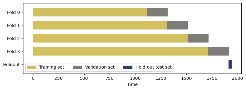
Great care must be taken when defining cross-validation folds for time-series data. We are not allowed to use the future to predict the past, so the training set must precede (in time) the validation set. Consequently, we partition the data set in the time dimension and assign the training and validation sets using time ranges:
# Cross-validation folds and held-out test set (in time dimension)
# The held-out test set is used for final evaluation
cv_folds = [  # (train_set, validation_set)
    ([0, 1114], [1114, 1314]),
    ([0, 1314], [1314, 1514]),
    ([0, 1514], [1514, 1714]),
    ([0, 1714], [1714, 1914]),
]
n_folds = len(cv_folds)
holdout = [1914, 1942]
time_horizon = 1942
It is helpful to visualize the cross-validation folds using Matplotlib.
cv_cmap = matplotlib.colormaps["cividis"]
plt.figure(figsize=(8, 3))

for i, (train_mask, valid_mask) in enumerate(cv_folds):
    idx = np.array([np.nan] * time_horizon)
    idx[np.arange(*train_mask)] = 1
    idx[np.arange(*valid_mask)] = 0
    plt.scatter(
        range(time_horizon),
        [i + 0.5] * time_horizon,
        c=idx,
        marker="_",
        capstyle="butt",
        s=1,
        lw=20,
        cmap=cv_cmap,
        vmin=-1.5,
        vmax=1.5,
    )

idx = np.array([np.nan] * time_horizon)
idx[np.arange(*holdout)] = -1
plt.scatter(
    range(time_horizon),
    [n_folds + 0.5] * time_horizon,
    c=idx,
    marker="_",
    capstyle="butt",
    s=1,
    lw=20,
    cmap=cv_cmap,
    vmin=-1.5,
    vmax=1.5,
)

plt.xlabel("Time")
plt.yticks(
    ticks=np.arange(n_folds + 1) + 0.5,
    labels=[f"Fold {i}" for i in range(n_folds)] + ["Holdout"],
)
plt.ylim([len(cv_folds) + 1.2, -0.2])

norm = matplotlib.colors.Normalize(vmin=-1.5, vmax=1.5)
plt.legend(
    [
        Patch(color=cv_cmap(norm(1))),
        Patch(color=cv_cmap(norm(0))),
        Patch(color=cv_cmap(norm(-1))),
    ],
    ["Training set", "Validation set", "Held-out test set"],
    ncol=3,
    loc="best",
)
plt.tight_layout()
Launch a Dask client on Kubernetes#
Let us set up a Dask cluster using the KubeCluster class.
cluster = KubeCluster(
    name="rapids-dask",
    image=rapids_image,
    worker_command="dask-cuda-worker",
    n_workers=n_workers,
    resources={"limits": {"nvidia.com/gpu": "1"}},
    env={"EXTRA_PIP_PACKAGES": "optuna gcsfs"},
)
cluster
client = Client(cluster)
client
Client
Client-dcc90a0f-5e32-11ee-8529-fa610e3dbb88
| Connection method: Cluster object | Cluster type: dask_kubernetes.KubeCluster |
| Dashboard: http://rapids-dask-scheduler.kubeflow-user-example-com:8787/status |
Cluster Info
KubeCluster
rapids-dask
| Dashboard: http://rapids-dask-scheduler.kubeflow-user-example-com:8787/status | Workers: 1 |
| Total threads: 1 | Total memory: 83.48 GiB |
Scheduler Info
Scheduler
Scheduler-ca08b554-394b-419d-b380-7b3ccdfd882f
| Comm: tcp://10.36.0.26:8786 | Workers: 1 |
| Dashboard: http://10.36.0.26:8787/status | Total threads: 1 |
| Started: Just now | Total memory: 83.48 GiB |
Workers
Worker: rapids-dask-default-worker-4f5ea8bc10
| Comm: tcp://10.36.2.23:34385 | Total threads: 1 |
| Dashboard: http://10.36.2.23:8788/status | Memory: 83.48 GiB |
| Nanny: tcp://10.36.2.23:44783 | |
| Local directory: /tmp/dask-scratch-space/worker-h2_cxa0d | |
| GPU: NVIDIA A100-SXM4-40GB | GPU memory: 40.00 GiB |
Define the custom evaluation metric#
The M5 forecasting competition defines a custom metric called WRMSSE as follows:
i.e. WRMSEE is a weighted sum of RMSSE for all product items \(i\). RMSSE is in turn defined to be
where the squared error of the prediction (forecast) is normalized by the speed at which the sales amount changes per unit in the training data.
Here is the implementation of the WRMSSE using cuDF. We use the product weights \(w_i\) as computed in the first preprocessing notebook.
def wrmsse(product_weights, df, pred_sales, train_mask, valid_mask):
    """Compute WRMSSE metric"""
    df_train = df[(df["day_id"] >= train_mask[0]) & (df["day_id"] < train_mask[1])]
    df_valid = df[(df["day_id"] >= valid_mask[0]) & (df["day_id"] < valid_mask[1])]

    # Compute denominator: 1/(n-1) * sum( (y(t) - y(t-1))**2 )
    diff = (
        df_train.sort_values(["item_id", "day_id"])
        .groupby(["item_id"])[["sales"]]
        .diff(1)
    )
    x = (
        df_train[["item_id", "day_id"]]
        .join(diff, how="left")
        .rename(columns={"sales": "diff"})
        .sort_values(["item_id", "day_id"])
    )
    x["diff"] = x["diff"] ** 2
    xx = x.groupby(["item_id"])[["diff"]].agg(["sum", "count"]).sort_index()
    xx.columns = xx.columns.map("_".join)
    xx["denominator"] = xx["diff_sum"] / xx["diff_count"]
    xx.reset_index()

    # Compute numerator: 1/h * sum( (y(t) - y_pred(t))**2 )
    X_valid = df_valid.drop(columns=["item_id", "cat_id", "day_id", "sales"])
    if "dept_id" in X_valid.columns:
        X_valid = X_valid.drop(columns=["dept_id"])
    df_pred = cudf.DataFrame(
        {
            "item_id": df_valid["item_id"].copy(),
            "pred_sales": pred_sales,
            "sales": df_valid["sales"].copy(),
        }
    )
    df_pred["diff"] = (df_pred["sales"] - df_pred["pred_sales"]) ** 2
    yy = df_pred.groupby(["item_id"])[["diff"]].agg(["sum", "count"]).sort_index()
    yy.columns = yy.columns.map("_".join)
    yy["numerator"] = yy["diff_sum"] / yy["diff_count"]

    zz = yy[["numerator"]].join(xx[["denominator"]], how="left")
    zz = zz.join(product_weights, how="left").sort_index()
    # Filter out zero denominator.
    # This can occur if the product was never on sale during the period in the training set
    zz = zz[zz["denominator"] != 0]
    zz["rmsse"] = np.sqrt(zz["numerator"] / zz["denominator"])
    return zz["rmsse"].multiply(zz["weights"]).sum()
Define the training and hyperparameter search pipeline using Optuna#
Optuna lets us define the training procedure iteratively, i.e. as if we were to write an ordinary function to train a single model. Instead of a fixed hyperparameter combination, the function now takes in a trial object which yields different hyperparameter combinations.
In this example, we partition the training data according to the store and then fit a separate XGBoost model per data segment.
def objective(trial):
    fs = gcsfs.GCSFileSystem()
    with fs.open(f"{bucket_name}/product_weights.pkl", "rb") as f:
        product_weights = cudf.DataFrame(pd.read_pickle(f))
    params = {
        "n_estimators": 100,
        "verbosity": 0,
        "learning_rate": 0.01,
        "objective": "reg:tweedie",
        "tree_method": "gpu_hist",
        "grow_policy": "depthwise",
        "predictor": "gpu_predictor",
        "enable_categorical": True,
        "lambda": trial.suggest_float("lambda", 1e-8, 100.0, log=True),
        "alpha": trial.suggest_float("alpha", 1e-8, 100.0, log=True),
        "colsample_bytree": trial.suggest_float("colsample_bytree", 0.2, 1.0),
        "max_depth": trial.suggest_int("max_depth", 2, 6, step=1),
        "min_child_weight": trial.suggest_float(
            "min_child_weight", 1e-8, 100, log=True
        ),
        "gamma": trial.suggest_float("gamma", 1e-8, 1.0, log=True),
        "tweedie_variance_power": trial.suggest_float("tweedie_variance_power", 1, 2),
    }
    scores = [[] for store in STORES]

    for store_id, store in enumerate(STORES):
        print(f"Processing store {store}...")
        with fs.open(f"{bucket_name}/combined_df_store_{store}.pkl", "rb") as f:
            df = cudf.DataFrame(pd.read_pickle(f))
        for train_mask, valid_mask in cv_folds:
            df_train = df[
                (df["day_id"] >= train_mask[0]) & (df["day_id"] < train_mask[1])
            ]
            df_valid = df[
                (df["day_id"] >= valid_mask[0]) & (df["day_id"] < valid_mask[1])
            ]

            X_train, y_train = (
                df_train.drop(
                    columns=["item_id", "dept_id", "cat_id", "day_id", "sales"]
                ),
                df_train["sales"],
            )
            X_valid = df_valid.drop(
                columns=["item_id", "dept_id", "cat_id", "day_id", "sales"]
            )

            clf = xgb.XGBRegressor(**params)
            clf.fit(X_train, y_train)
            pred_sales = clf.predict(X_valid)
            scores[store_id].append(
                wrmsse(product_weights, df, pred_sales, train_mask, valid_mask)
            )
            del df_train, df_valid, X_train, y_train, clf
            gc.collect()
        del df
        gc.collect()

    # We can sum WRMSSE scores over data segments because data segments contain disjoint sets of time series
    return np.array(scores).sum(axis=0).mean()
Using the Dask cluster client, we execute multiple training jobs in parallel. Optuna keeps track of the progress in the hyperparameter search using in-memory Dask storage.
##### Number of hyperparameter combinations to try in parallel
n_trials = 9  # Using a small n_trials so that the demo can finish quickly
# n_trials = 100

# Optimize in parallel on your Dask cluster
backend_storage = optuna.storages.InMemoryStorage()
dask_storage = optuna.integration.DaskStorage(storage=backend_storage, client=client)
study = optuna.create_study(
    direction="minimize",
    sampler=optuna.samplers.RandomSampler(seed=0),
    storage=dask_storage,
)
futures = []
for i in range(0, n_trials, n_workers):
    iter_range = (i, min([i + n_workers, n_trials]))
    futures.append(
        {
            "range": iter_range,
            "futures": [
                client.submit(
                    # Work around bug https://github.com/optuna/optuna/issues/4859
                    lambda objective, n_trials: (
                        study.sampler.reseed_rng(),
                        study.optimize(objective, n_trials),
                    ),
                    objective,
                    n_trials=1,
                    pure=False,
                )
                for _ in range(*iter_range)
            ],
        }
    )

tstart = time.perf_counter()
for partition in futures:
    iter_range = partition["range"]
    print(f"Testing hyperparameter combinations {iter_range[0]}..{iter_range[1]}")
    _ = wait(partition["futures"])
    for fut in partition["futures"]:
        _ = fut.result()  # Ensure that the training job was successful
    tnow = time.perf_counter()
    print(
        f"Best cross-validation metric: {study.best_value}, Time elapsed = {tnow - tstart}"
    )
tend = time.perf_counter()
print(f"Total time elapsed = {tend - tstart}")
/tmp/ipykernel_1321/3389696366.py:7: ExperimentalWarning: DaskStorage is experimental (supported from v3.1.0). The interface can change in the future.
  dask_storage = optuna.integration.DaskStorage(storage=backend_storage, client=client)
Testing hyperparameter combinations 0..2
Best cross-validation metric: 10.027767173304472, Time elapsed = 331.6198390149948
Testing hyperparameter combinations 2..4
Best cross-validation metric: 9.426913749927916, Time elapsed = 640.7606940959959
Testing hyperparameter combinations 4..6
Best cross-validation metric: 9.426913749927916, Time elapsed = 958.0816706369951
Testing hyperparameter combinations 6..8
Best cross-validation metric: 9.426913749927916, Time elapsed = 1295.700604706988
Testing hyperparameter combinations 8..9
Best cross-validation metric: 8.915009508695244, Time elapsed = 1476.1182343699911
Total time elapsed = 1476.1219055669935
Once the hyperparameter search is complete, we fetch the optimal hyperparameter combination using the attributes of the study object.
study.best_params
{'lambda': 2.6232990699579064e-06,
 'alpha': 0.004085800094564677,
 'colsample_bytree': 0.4064535567263888,
 'max_depth': 6,
 'min_child_weight': 9.652128310148716e-08,
 'gamma': 3.4446109254037165e-07,
 'tweedie_variance_power': 1.0914258082324833}
study.best_trial
FrozenTrial(number=8, state=TrialState.COMPLETE, values=[8.915009508695244], datetime_start=datetime.datetime(2023, 9, 28, 19, 35, 29, 888497), datetime_complete=datetime.datetime(2023, 9, 28, 19, 38, 30, 299541), params={'lambda': 2.6232990699579064e-06, 'alpha': 0.004085800094564677, 'colsample_bytree': 0.4064535567263888, 'max_depth': 6, 'min_child_weight': 9.652128310148716e-08, 'gamma': 3.4446109254037165e-07, 'tweedie_variance_power': 1.0914258082324833}, user_attrs={}, system_attrs={}, intermediate_values={}, distributions={'lambda': FloatDistribution(high=100.0, log=True, low=1e-08, step=None), 'alpha': FloatDistribution(high=100.0, log=True, low=1e-08, step=None), 'colsample_bytree': FloatDistribution(high=1.0, log=False, low=0.2, step=None), 'max_depth': IntDistribution(high=6, log=False, low=2, step=1), 'min_child_weight': FloatDistribution(high=100.0, log=True, low=1e-08, step=None), 'gamma': FloatDistribution(high=1.0, log=True, low=1e-08, step=None), 'tweedie_variance_power': FloatDistribution(high=2.0, log=False, low=1.0, step=None)}, trial_id=8, value=None)
# Make a deep copy to preserve the dictionary after deleting the Dask cluster
best_params = copy.deepcopy(study.best_params)
best_params
{'lambda': 2.6232990699579064e-06,
 'alpha': 0.004085800094564677,
 'colsample_bytree': 0.4064535567263888,
 'max_depth': 6,
 'min_child_weight': 9.652128310148716e-08,
 'gamma': 3.4446109254037165e-07,
 'tweedie_variance_power': 1.0914258082324833}
fs = gcsfs.GCSFileSystem()
with fs.open(f"{bucket_name}/params.json", "w") as f:
    json.dump(best_params, f)
Train the final XGBoost model and evaluate#
Using the optimal hyperparameters found in the search, fit a new model using the whole training data. As in the previous section, we fit a separate XGBoost model per data segment.
fs = gcsfs.GCSFileSystem()
with fs.open(f"{bucket_name}/params.json", "r") as f:
    best_params = json.load(f)
with fs.open(f"{bucket_name}/product_weights.pkl", "rb") as f:
    product_weights = cudf.DataFrame(pd.read_pickle(f))
def final_train(best_params):
    fs = gcsfs.GCSFileSystem()
    params = {
        "n_estimators": 100,
        "verbosity": 0,
        "learning_rate": 0.01,
        "objective": "reg:tweedie",
        "tree_method": "gpu_hist",
        "grow_policy": "depthwise",
        "predictor": "gpu_predictor",
        "enable_categorical": True,
    }
    params.update(best_params)
    model = {}
    train_mask = [0, 1914]

    for store in STORES:
        print(f"Processing store {store}...")
        with fs.open(f"{bucket_name}/combined_df_store_{store}.pkl", "rb") as f:
            df = cudf.DataFrame(pd.read_pickle(f))

        df_train = df[(df["day_id"] >= train_mask[0]) & (df["day_id"] < train_mask[1])]
        X_train, y_train = (
            df_train.drop(columns=["item_id", "dept_id", "cat_id", "day_id", "sales"]),
            df_train["sales"],
        )

        clf = xgb.XGBRegressor(**params)
        clf.fit(X_train, y_train)
        model[store] = clf
    del df
    gc.collect()

    return model
model = final_train(best_params)
Processing store CA_1...
Processing store CA_2...
Processing store CA_3...
Processing store CA_4...
Processing store TX_1...
Processing store TX_2...
Processing store TX_3...
Processing store WI_1...
Processing store WI_2...
Processing store WI_3...
Let’s now evaluate the final model using the held-out test set:
test_wrmsse = 0
for store in STORES:
    with fs.open(f"{bucket_name}/combined_df_store_{store}.pkl", "rb") as f:
        df = cudf.DataFrame(pd.read_pickle(f))
    df_test = df[(df["day_id"] >= holdout[0]) & (df["day_id"] < holdout[1])]
    X_test = df_test.drop(columns=["item_id", "dept_id", "cat_id", "day_id", "sales"])
    pred_sales = model[store].predict(X_test)
    test_wrmsse += wrmsse(
        product_weights, df, pred_sales, train_mask=[0, 1914], valid_mask=holdout
    )
print(f"WRMSSE metric on the held-out test set: {test_wrmsse}")
WRMSSE metric on the held-out test set: 9.478942050051291
# Save the model to the Cloud Storage
with fs.open(f"{bucket_name}/final_model.pkl", "wb") as f:
    pickle.dump(model, f)
Create an ensemble model using a different strategy for segmenting sales data#
It is common to create an ensemble model where multiple machine learning methods are used to obtain better predictive performance. Prediction is made from an ensemble model by averaging the prediction output of the constituent models.
In this example, we will create a second model by segmenting the sales data in a different way. Instead of splitting by stores, we will split the data by both stores and product categories.
def objective_alt(trial):
    fs = gcsfs.GCSFileSystem()
    with fs.open(f"{bucket_name}/product_weights.pkl", "rb") as f:
        product_weights = cudf.DataFrame(pd.read_pickle(f))
    params = {
        "n_estimators": 100,
        "verbosity": 0,
        "learning_rate": 0.01,
        "objective": "reg:tweedie",
        "tree_method": "gpu_hist",
        "grow_policy": "depthwise",
        "predictor": "gpu_predictor",
        "enable_categorical": True,
        "lambda": trial.suggest_float("lambda", 1e-8, 100.0, log=True),
        "alpha": trial.suggest_float("alpha", 1e-8, 100.0, log=True),
        "colsample_bytree": trial.suggest_float("colsample_bytree", 0.2, 1.0),
        "max_depth": trial.suggest_int("max_depth", 2, 6, step=1),
        "min_child_weight": trial.suggest_float(
            "min_child_weight", 1e-8, 100, log=True
        ),
        "gamma": trial.suggest_float("gamma", 1e-8, 1.0, log=True),
        "tweedie_variance_power": trial.suggest_float("tweedie_variance_power", 1, 2),
    }
    scores = [[] for i in range(len(STORES) * len(DEPTS))]

    for store_id, store in enumerate(STORES):
        for dept_id, dept in enumerate(DEPTS):
            print(f"Processing store {store}, department {dept}...")
            with fs.open(
                f"{bucket_name}/combined_df_store_{store}_dept_{dept}.pkl", "rb"
            ) as f:
                df = cudf.DataFrame(pd.read_pickle(f))
            for train_mask, valid_mask in cv_folds:
                df_train = df[
                    (df["day_id"] >= train_mask[0]) & (df["day_id"] < train_mask[1])
                ]
                df_valid = df[
                    (df["day_id"] >= valid_mask[0]) & (df["day_id"] < valid_mask[1])
                ]

                X_train, y_train = (
                    df_train.drop(columns=["item_id", "cat_id", "day_id", "sales"]),
                    df_train["sales"],
                )
                X_valid = df_valid.drop(
                    columns=["item_id", "cat_id", "day_id", "sales"]
                )

                clf = xgb.XGBRegressor(**params)
                clf.fit(X_train, y_train)
                sales_pred = clf.predict(X_valid)
                scores[store_id * len(DEPTS) + dept_id].append(
                    wrmsse(product_weights, df, sales_pred, train_mask, valid_mask)
                )
                del df_train, df_valid, X_train, y_train, clf
                gc.collect()
            del df
            gc.collect()

    # We can sum WRMSSE scores over data segments because data segments contain disjoint sets of time series
    return np.array(scores).sum(axis=0).mean()
##### Number of hyperparameter combinations to try in parallel
n_trials = 9  # Using a small n_trials so that the demo can finish quickly
# n_trials = 100

# Optimize in parallel on your Dask cluster
backend_storage = optuna.storages.InMemoryStorage()
dask_storage = optuna.integration.DaskStorage(storage=backend_storage, client=client)
study = optuna.create_study(
    direction="minimize",
    sampler=optuna.samplers.RandomSampler(seed=0),
    storage=dask_storage,
)
futures = []
for i in range(0, n_trials, n_workers):
    iter_range = (i, min([i + n_workers, n_trials]))
    futures.append(
        {
            "range": iter_range,
            "futures": [
                client.submit(
                    # Work around bug https://github.com/optuna/optuna/issues/4859
                    lambda objective, n_trials: (
                        study.sampler.reseed_rng(),
                        study.optimize(objective, n_trials),
                    ),
                    objective_alt,
                    n_trials=1,
                    pure=False,
                )
                for _ in range(*iter_range)
            ],
        }
    )

tstart = time.perf_counter()
for partition in futures:
    iter_range = partition["range"]
    print(f"Testing hyperparameter combinations {iter_range[0]}..{iter_range[1]}")
    _ = wait(partition["futures"])
    for fut in partition["futures"]:
        _ = fut.result()  # Ensure that the training job was successful
    tnow = time.perf_counter()
    print(
        f"Best cross-validation metric: {study.best_value}, Time elapsed = {tnow - tstart}"
    )
tend = time.perf_counter()
print(f"Total time elapsed = {tend - tstart}")
/tmp/ipykernel_1321/491731696.py:7: ExperimentalWarning: DaskStorage is experimental (supported from v3.1.0). The interface can change in the future.
  dask_storage = optuna.integration.DaskStorage(storage=backend_storage, client=client)
Testing hyperparameter combinations 0..2
Best cross-validation metric: 9.896445497438858, Time elapsed = 802.2191872399999
Testing hyperparameter combinations 2..4
Best cross-validation metric: 9.896445497438858, Time elapsed = 1494.0718872279976
Testing hyperparameter combinations 4..6
Best cross-validation metric: 9.835407407395302, Time elapsed = 2393.3159628150024
Testing hyperparameter combinations 6..8
Best cross-validation metric: 9.330048901795887, Time elapsed = 3092.471466117
Testing hyperparameter combinations 8..9
Best cross-validation metric: 9.330048901795887, Time elapsed = 3459.9082761530008
Total time elapsed = 3459.911843854992
# Make a deep copy to preserve the dictionary after deleting the Dask cluster
best_params_alt = copy.deepcopy(study.best_params)
best_params_alt
{'lambda': 0.028794929327421122,
 'alpha': 3.3150619134761685e-07,
 'colsample_bytree': 0.42330433646728755,
 'max_depth': 2,
 'min_child_weight': 0.09713314395591004,
 'gamma': 0.0016337599227941016,
 'tweedie_variance_power': 1.1915217521234043}
fs = gcsfs.GCSFileSystem()
with fs.open(f"{bucket_name}/params_alt.json", "w") as f:
    json.dump(best_params_alt, f)
Using the optimal hyperparameters found in the search, fit a new model using the whole training data.
def final_train_alt(best_params):
    fs = gcsfs.GCSFileSystem()
    params = {
        "n_estimators": 100,
        "verbosity": 0,
        "learning_rate": 0.01,
        "objective": "reg:tweedie",
        "tree_method": "gpu_hist",
        "grow_policy": "depthwise",
        "predictor": "gpu_predictor",
        "enable_categorical": True,
    }
    params.update(best_params)
    model = {}
    train_mask = [0, 1914]

    for _, store in enumerate(STORES):
        for _, dept in enumerate(DEPTS):
            print(f"Processing store {store}, department {dept}...")
            with fs.open(
                f"{bucket_name}/combined_df_store_{store}_dept_{dept}.pkl", "rb"
            ) as f:
                df = cudf.DataFrame(pd.read_pickle(f))
            for train_mask, _ in cv_folds:
                df_train = df[
                    (df["day_id"] >= train_mask[0]) & (df["day_id"] < train_mask[1])
                ]
                X_train, y_train = (
                    df_train.drop(columns=["item_id", "cat_id", "day_id", "sales"]),
                    df_train["sales"],
                )

                clf = xgb.XGBRegressor(**params)
                clf.fit(X_train, y_train)
                model[(store, dept)] = clf
            del df
            gc.collect()

    return model
fs = gcsfs.GCSFileSystem()
with fs.open(f"{bucket_name}/params_alt.json", "r") as f:
    best_params_alt = json.load(f)
with fs.open(f"{bucket_name}/product_weights.pkl", "rb") as f:
    product_weights = cudf.DataFrame(pd.read_pickle(f))
model_alt = final_train_alt(best_params_alt)
Processing store CA_1, department HOBBIES_1...
Processing store CA_1, department HOBBIES_2...
Processing store CA_1, department HOUSEHOLD_1...
Processing store CA_1, department HOUSEHOLD_2...
Processing store CA_1, department FOODS_1...
Processing store CA_1, department FOODS_2...
Processing store CA_1, department FOODS_3...
Processing store CA_2, department HOBBIES_1...
Processing store CA_2, department HOBBIES_2...
Processing store CA_2, department HOUSEHOLD_1...
Processing store CA_2, department HOUSEHOLD_2...
Processing store CA_2, department FOODS_1...
Processing store CA_2, department FOODS_2...
Processing store CA_2, department FOODS_3...
Processing store CA_3, department HOBBIES_1...
Processing store CA_3, department HOBBIES_2...
Processing store CA_3, department HOUSEHOLD_1...
Processing store CA_3, department HOUSEHOLD_2...
Processing store CA_3, department FOODS_1...
Processing store CA_3, department FOODS_2...
Processing store CA_3, department FOODS_3...
Processing store CA_4, department HOBBIES_1...
Processing store CA_4, department HOBBIES_2...
Processing store CA_4, department HOUSEHOLD_1...
Processing store CA_4, department HOUSEHOLD_2...
Processing store CA_4, department FOODS_1...
Processing store CA_4, department FOODS_2...
Processing store CA_4, department FOODS_3...
Processing store TX_1, department HOBBIES_1...
Processing store TX_1, department HOBBIES_2...
Processing store TX_1, department HOUSEHOLD_1...
Processing store TX_1, department HOUSEHOLD_2...
Processing store TX_1, department FOODS_1...
Processing store TX_1, department FOODS_2...
Processing store TX_1, department FOODS_3...
Processing store TX_2, department HOBBIES_1...
Processing store TX_2, department HOBBIES_2...
Processing store TX_2, department HOUSEHOLD_1...
Processing store TX_2, department HOUSEHOLD_2...
Processing store TX_2, department FOODS_1...
Processing store TX_2, department FOODS_2...
Processing store TX_2, department FOODS_3...
Processing store TX_3, department HOBBIES_1...
Processing store TX_3, department HOBBIES_2...
Processing store TX_3, department HOUSEHOLD_1...
Processing store TX_3, department HOUSEHOLD_2...
Processing store TX_3, department FOODS_1...
Processing store TX_3, department FOODS_2...
Processing store TX_3, department FOODS_3...
Processing store WI_1, department HOBBIES_1...
Processing store WI_1, department HOBBIES_2...
Processing store WI_1, department HOUSEHOLD_1...
Processing store WI_1, department HOUSEHOLD_2...
Processing store WI_1, department FOODS_1...
Processing store WI_1, department FOODS_2...
Processing store WI_1, department FOODS_3...
Processing store WI_2, department HOBBIES_1...
Processing store WI_2, department HOBBIES_2...
Processing store WI_2, department HOUSEHOLD_1...
Processing store WI_2, department HOUSEHOLD_2...
Processing store WI_2, department FOODS_1...
Processing store WI_2, department FOODS_2...
Processing store WI_2, department FOODS_3...
Processing store WI_3, department HOBBIES_1...
Processing store WI_3, department HOBBIES_2...
Processing store WI_3, department HOUSEHOLD_1...
Processing store WI_3, department HOUSEHOLD_2...
Processing store WI_3, department FOODS_1...
Processing store WI_3, department FOODS_2...
Processing store WI_3, department FOODS_3...
# Save the model to the Cloud Storage
with fs.open(f"{bucket_name}/final_model_alt.pkl", "wb") as f:
    pickle.dump(model_alt, f)
Now consider an ensemble consisting of the two models model and model_alt. We evaluate the ensemble by computing the WRMSSE metric for the average of the predictions of the two models.
test_wrmsse = 0
for store in STORES:
    print(f"Processing store {store}...")
    # Prediction from Model 1
    with fs.open(f"{bucket_name}/combined_df_store_{store}.pkl", "rb") as f:
        df = cudf.DataFrame(pd.read_pickle(f))
    df_test = df[(df["day_id"] >= holdout[0]) & (df["day_id"] < holdout[1])]
    X_test = df_test.drop(columns=["item_id", "dept_id", "cat_id", "day_id", "sales"])
    df_test["pred1"] = model[store].predict(X_test)

    # Prediction from Model 2
    df_test["pred2"] = [np.nan] * len(df_test)
    df_test["pred2"] = df_test["pred2"].astype("float32")
    for dept in DEPTS:
        with fs.open(
            f"{bucket_name}/combined_df_store_{store}_dept_{dept}.pkl", "rb"
        ) as f:
            df2 = cudf.DataFrame(pd.read_pickle(f))
        df2_test = df2[(df2["day_id"] >= holdout[0]) & (df2["day_id"] < holdout[1])]
        X_test = df2_test.drop(columns=["item_id", "cat_id", "day_id", "sales"])
        assert np.sum(df_test["dept_id"] == dept) == len(X_test)
        df_test["pred2"][df_test["dept_id"] == dept] = model_alt[(store, dept)].predict(
            X_test
        )

    # Average prediction
    df_test["avg_pred"] = (df_test["pred1"] + df_test["pred2"]) / 2.0

    test_wrmsse += wrmsse(
        product_weights,
        df,
        df_test["avg_pred"],
        train_mask=[0, 1914],
        valid_mask=holdout,
    )
print(f"WRMSSE metric on the held-out test set: {test_wrmsse}")
Processing store CA_1...
Processing store CA_2...
Processing store CA_3...
Processing store CA_4...
Processing store TX_1...
Processing store TX_2...
Processing store TX_3...
Processing store WI_1...
Processing store WI_2...
Processing store WI_3...
WRMSSE metric on the held-out test set: 10.69187847848366
# Close the Dask cluster to clean up
cluster.close()
Conclusion#
We demonstrated an end-to-end workflow where we take a real-world time-series data and train a forecasting model using Google Kubernetes Engine (GKE). We were able to speed up the hyperparameter optimization (HPO) process by dispatching parallel training jobs to NVIDIA GPUs.