Measuring performance with the One Billion Row Challenge#

The One Billion Row Challenge is a programming competition aimed at Java developers to write the most efficient code to process a one billion line text file and calculate some metrics. The challenge has inspired solutions in many languages beyond Java including Python.

In this notebook we will explore how we can use RAPIDS to build an efficient solution in Python and how we can use dashboards to understand how performant our code is.

The Problem#

The input data of the challenge is a ~13GB text file containing one billion lines of temperature measurements. The file is structured with one measurement per line with the name of the weather station and the measurement separated by a semicolon.

Hamburg;12.0
Bulawayo;8.9
Palembang;38.8
St. John's;15.2
Cracow;12.6
...

Our goal is to calculate the min, mean, and max temperature per weather station sorted alphabetically by station name as quickly as possible.

Reference implementation#

A reference implementation written with popular PyData tools would likely be something along the lines of the following Pandas code (assuming you have enough RAM to fit the data into memory).

import pandas as pd

df = pd.read_csv(
    "measurements.txt",
    sep=";",
    header=None,
    names=["station", "measure"],
    engine='pyarrow'
)
df = df.groupby("station").agg(["min", "max", "mean"])
df.columns = df.columns.droplevel()
df = df.sort_values("station")

Here we use pandas.read_csv() to open the text file and specify the ; separator and also set some column names. We also set the engine to pyarrow to give us some extra performance out of the box.

Then we group the measurements by their station name and calculate the min, max and mean. Finally we sort the grouped dataframe by the station name.

Running this on a workstation with a 12-core CPU completes the task in around 4 minutes.

Deploying RAPIDS#

To run this notebook we will need a machine with one or more GPUs. There are many ways you can get this:

Have a laptop, desktop or workstation with GPUs.
Run a VM on the cloud using AWS EC2, Google Compute Engine, Azure VMs, etc.
Use a managed notebook service like SageMaker, Vertex AI, Azure ML or Databricks.
Run a container in a Kubernetes cluster with GPUs.

Once you have a GPU machine you will need to install RAPIDS. You can do this with pip, conda or docker.

We are also going to use Jupyter Lab with the RAPIDS nvdashboard extension and the Dask Lab Extension so that we can understand what our machine is doing. If you are using the Docker container these will already be installed for you, otherwise you will need to install them yourself.

Dashboards#

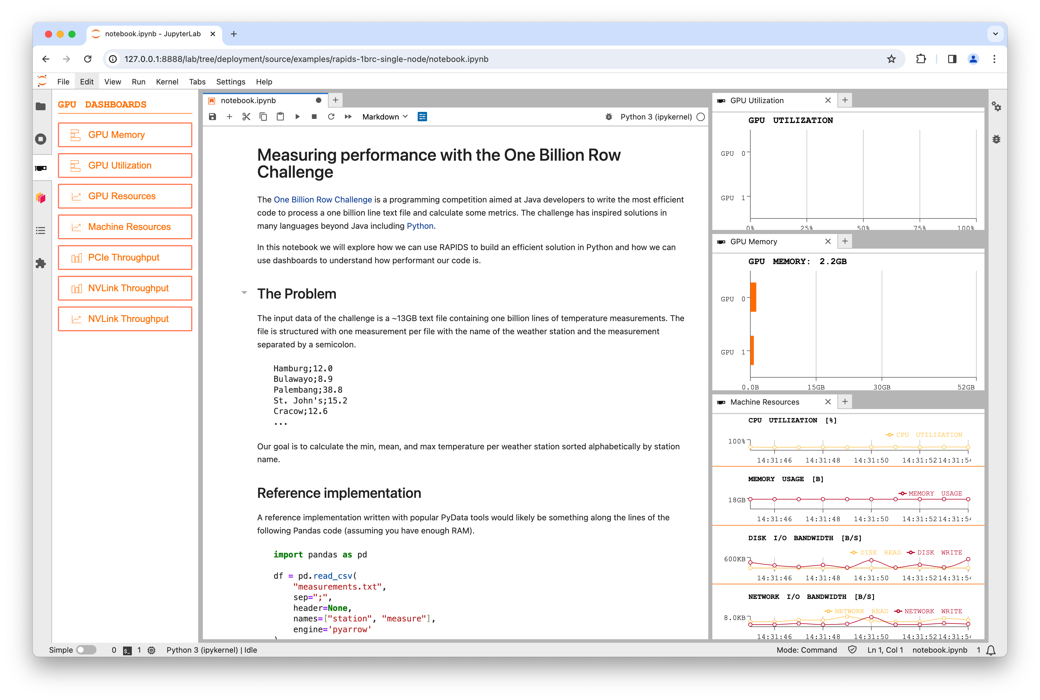
Once you have Jupyter up and running with the extensions installed and this notebook downloaded you can open some performance dashboards so we can monitor our hardware as our code runs.

Let’s start with nvdashboard which has the GPU icon in the left toolbar.

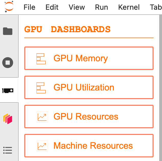
Start by opening the “Machine Resources” table, “GPU Utilization” graph and “GPU Memory” graph and moving them over to the right hand side.

Data Generation#

Before we get started with our problem we need to generate the input data. The 1BRC repo has a Java implementation which takes around 15 minutes to generate the file.

If you were to run the Java implementation you would see the CPU get busy but disk bandwidth remain low, suggesting this is a compute bound problem. We can accelerate this on the GPU using cuDF and CuPy.

Download the lookup.csv table of stations and their mean temperatures as we will use this to generate our data file containing n rows of random temperatures.

To generate each row we choose a random station from the lookup table, then generate a random temperature measurement from a normal distribution around the mean temp. We assume the standard deviation is 10.0 for all stations.

import cupy as cp
import cudf
from pathlib import Path
import time

def generate_chunk(filename, chunksize, std, lookup_df):
    """Generate some sample data based on the lookup table."""
    df = cudf.DataFrame(
        {
            # Choose a random station from the lookup table for each row in our output
            "station": cp.random.randint(0, len(lookup_df) - 1, int(chunksize)),
            # Generate a normal distibution around zero for each row in our output
            # Because the std is the same for every station we can adjust the mean for each row afterwards
            "measure": cp.random.normal(0, std, int(chunksize)),
        }
    )

    # Offset each measurement by the station's mean value
    df.measure += df.station.map(lookup_df.mean_temp)
    # Round the temprature to one decimal place
    df.measure = df.measure.round(decimals=1)
    # Convert the station index to the station name
    df.station = df.station.map(lookup_df.station)

    # Append this chunk to the output file
    with open(filename, "a") as fh:
        df.to_csv(fh, sep=";", chunksize=10_000_000, header=False, index=False)

Configuration#

n = 1_000_000_000  # Number of rows of data to generate

lookup_df = cudf.read_csv(
    "lookup.csv"
)  # Load our lookup table of stations and their mean temperatures
std = 10.0  # We assume temperatures are normally distributed with a standard deviation of 10
chunksize = 2e8  # Set the number of rows to generate in one go (reduce this if you run into GPU RAM limits)
filename = Path(f"measurements.txt")  # Choose where to write to
filename.unlink() if filename.exists() else None  # Delete the file if it exists already

Run the data generation#

%%time
# Loop over chunks and generate data
start = time.time()
for i in range(int(n / chunksize)):
    # Generate a chunk
    generate_chunk(filename, chunksize, std, lookup_df)

    # Update the progress bar
    percent_complete = int(((i + 1) * chunksize) / n * 100)
    time_taken = int(time.time() - start)
    time_remaining = int((time_taken / percent_complete) * 100) - time_taken
    print(
        f"Writing {int(n / 1e9)} billion rows to {filename}: {percent_complete}% in {time_taken}s ({time_remaining}s remaining)",
        end="\r",
    )
print()

Writing 1 billion rows to measurements.txt: 100% in 25s (0s remaining)
CPU times: user 10.1 s, sys: 18 s, total: 28.2 s
Wall time: 25.3 s

If you watch the graphs while this cell is running you should see a burts of GPU utilization when the GPU generates the random numbers followed by a burst of Disk IO when that data is written to disk. This pattern will happen for each chunk that is generated.

Note

We could improve performance even further here by generating the next chunk while the current chunk is writing to disk, but a 30x speedup seems optimal enough for now.

Check the files#

Now we can verify our dataset is the size we expected and contains rows that follow the format needed by the challenge.

!ls -lh {filename}

-rw-r--r-- 1 rapids conda 13G Jan 22 16:54 measurements.txt

!head {filename}

Guatemala City;17.3
Launceston;24.3
Bulawayo;8.7
Tbilisi;9.5
Napoli;26.8
Sarajevo;27.5
Chihuahua;29.2
Ho Chi Minh City;8.4
Johannesburg;19.2
Cape Town;16.3

GPU solution with RAPIDS#

Now let’s look at using RAPIDS to speed up our Pandas implementation of the challenge. If you directly convert the reference implementation from Pandas to cuDF you will run into some limitations cuDF has with string columns. Also depending on your GPU you may run into memory limits as cuDF will read the whole dataset into memory and machines typically have less GPU memory than CPU memory.

Therefore to solve this with RAPIDS we also need to use Dask to partition the dataset and stream it through GPU memory, then cuDF can process each partition in a performant way.

Deploying Dask#

We are going to use dask-cuda to start a GPU Dask cluster.

from dask.distributed import Client
from dask_cuda import LocalCUDACluster

client = Client(LocalCUDACluster())

Creating a LocalCUDACluster() inspects the machine and starts one Dask worker for each detected GPU. We then pass that to a Dask client which means that all following code in the notebook will leverage the GPU workers.

Tip

Dask has a lot of different tools for deploying clusters, and they all follow the same format of instantiating a class. So whether you are trying to leverage all of the resources in a single machine like this example or trying to leverage an entire multi-node cluster Dask can get you up and running quickly.

Dask dashboard#

We can also make use of the Dask Dashboard to see what is going on.

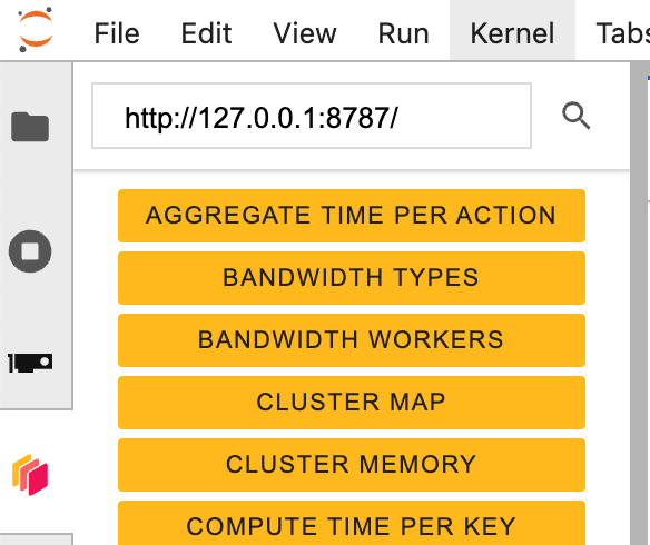
If you select the Dask logo from the left-hand toolbar and then click the search icon it should detect our LocalCUDACluster automatically and show us a long list of graphs to choose from.

When working with GPUs the “GPU Utilization” and “GPU Memory” will show us the same as the nvdashboard plots but for all machines in our Dask cluster. This is very helpful when working on a multi-node cluster but doesn’t help us in thie single-node configuration.

To see what Dask is doing in this challenge you should open the “Progress” and “Task Stream” graphs which will show all of the operations being performed. But feel free to open other graphs and explore all of the different metrics Dask can give you.

Dask + cuDF Solution#

Now that we have our input data and a Dask cluster we can write some Dask code that leverages cuDF under the hood to perform the compute operations.

First we need to import dask.dataframe and tell it to use the cudf backend.

import dask
import dask.dataframe as dd

dask.config.set({"dataframe.backend": "cudf"})

<dask.config.set at 0x7fbd773ae590>

Now we can run our Dask code, which is almost identical to the Pandas code we used before.

%%timeit -n 3 -r 4
df = dd.read_csv("measurements.txt", sep=";", header=None, names=["station", "measure"])
df = df.groupby("station").agg(["min", "max", "mean"])
df.columns = df.columns.droplevel()

# We need to switch back to Pandas for the final sort at the time of writing due to rapidsai/cudf#14794
df = df.compute().to_pandas()
df = df.sort_values("station")

4.59 s ± 124 ms per loop (mean ± std. dev. of 4 runs, 3 loops each)

Running this notebook on a desktop workstation with two NVIDIA RTX 8000 GPUs completes the challenge in around 4 seconds (a 60x speedup over Pandas).

Watching the progress bars you should see them fill and reset a total of 12 times as our %%timeit operation is solving the challenge multiple times to get an average speed.

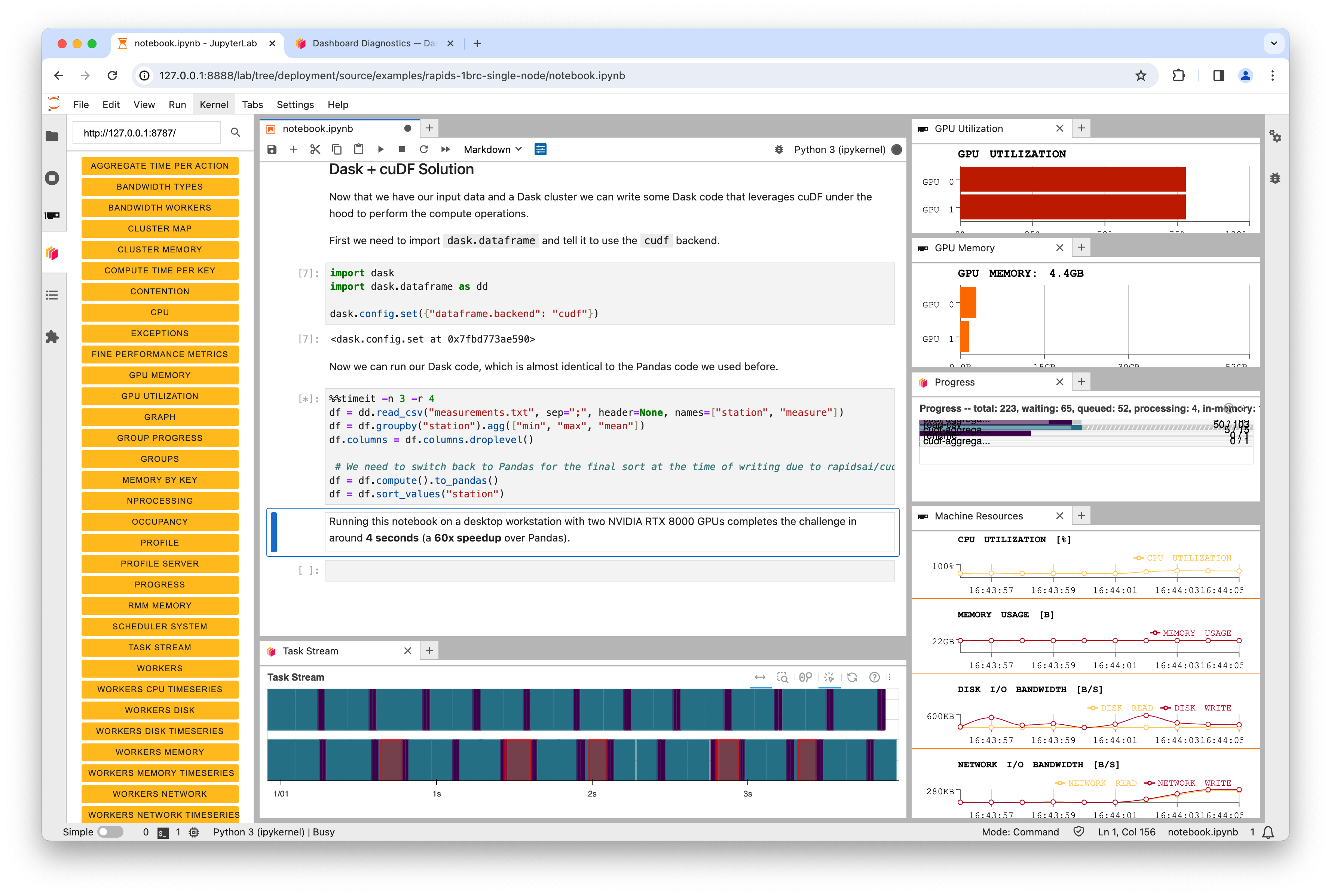
In the above screenshot you can see that on a dual-GPU system Dask was leveraging both GPUs. But it’s also interesting to note that the GPU utilization never reaches 100%. This is because the SSD in the machine has now become the bottleneck. The GPUs are performing the calculations so efficiently that we can’t read data from disk fast enough to fully saturate them.

Conclusion#

RAPIDS can accelerate existing workflows written with libraries like Pandas with little to no code changes. GPUs can accelerate computations by orders of magnitude which can move performance bottlenecks to other parts of the system.

Using dashboarding tools like nvdashboard and the Dask dashboard allow you to see and understand how your system is performing. Perhaps in this example upgrading the SSD is the next step to achieving even more performance.