Kubeflow

You can use RAPIDS with Kubeflow in a single pod with Kubeflow Notebooks or you can scale out to many pods on many nodes of the Kubernetes cluster with the dask-operator.

Note

These instructions were tested against Kubeflow v1.5.1 running on Kubernetes v1.21. Visit Installing Kubeflow for instructions on installing Kubeflow on your Kubernetes cluster.

Kubeflow Notebooks

The RAPIDS docker images can be used directly in Kubeflow Notebooks with no additional configuration. To find the latest image head to the RAPIDS install page, as shown in below, and choose a version of RAPIDS to use. Typically we want to choose the container image for the latest release. Verify the Docker image is selected when installing the latest RAPIDS release.

Be sure to match the CUDA version in the container image with that installed on your Kubernetes nodes. The default CUDA version installed on GKE Stable is 11.4 for example, so we would want to choose that. From 11.5 onwards it doesn’t matter as they will be backward compatible. Copy the container image name from the install command (i.e. nvcr.io/nvidia/rapidsai/base:24.04-cuda11.8-py3.10).

Note

You can check your CUDA version by creating a pod and running nvidia-smi. For example:

$ kubectl run nvidia-smi --restart=Never --rm -i --tty --image nvidia/cuda:11.0.3-base-ubuntu20.04 -- nvidia-smi
+-----------------------------------------------------------------------------+
| NVIDIA-SMI 495.46       Driver Version: 495.46       CUDA Version: 11.5     |
|-------------------------------+----------------------+----------------------+
...

Now in Kubeflow, access the Notebooks tab on the left and click “New Notebook”.

On this page, we must set a few configuration options. First, let’s give it a name like rapids. We need to check the “use custom image” box and paste in the container image we got from the RAPIDS release selector. Then, we want to set the CPU and RAM to something a little higher (i.e. 2 CPUs and 8GB memory) and set the number of NVIDIA GPUs to 1.

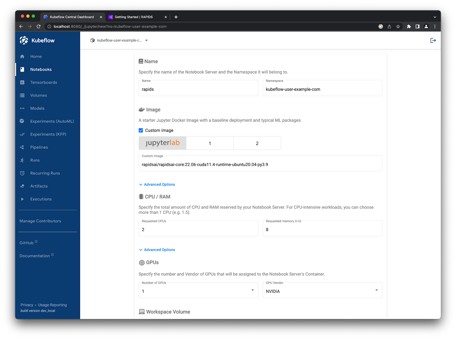
New Kubeflow notebook form named rapids with the custom RAPIDS container image, 2 CPU cores, 8GB of RAM, and 1 NVIDIA GPU selected

Then, you can scroll to the bottom of the page and hit launch. You should see it starting up in your list. The RAPIDS container images are packed full of amazing tools so this step can take a little while.

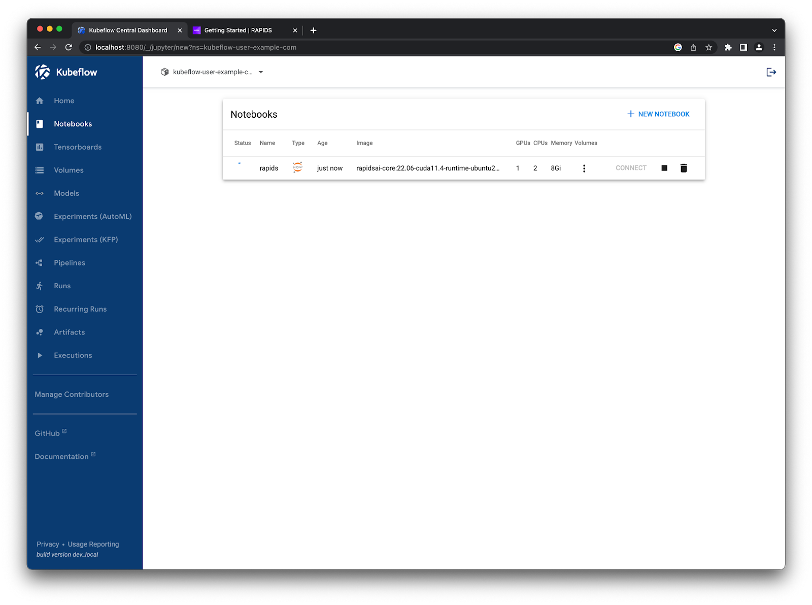
Once the Notebook is ready, click Connect to launch Jupyter.

You can verify everything works okay by opening a terminal in Jupyter and running:

$ nvidia-smi

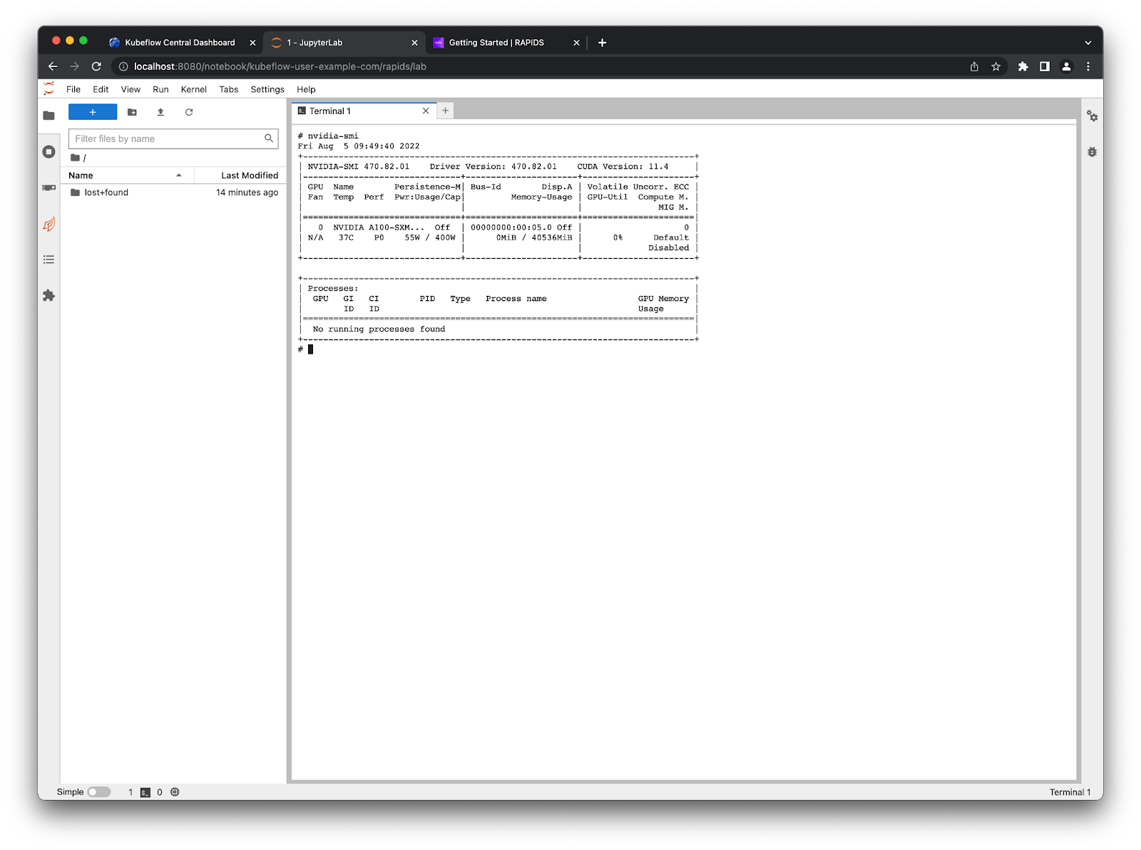
There is one A100 GPU listed which is available for use in your Notebook.

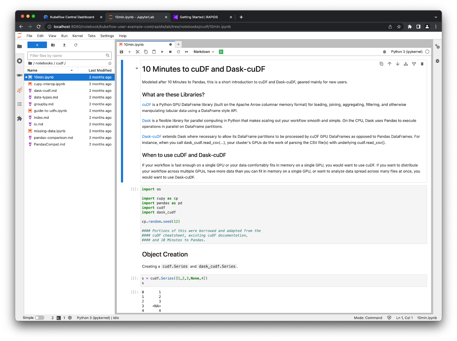
The RAPIDS container also comes with some example notebooks which you can find in /rapids/notebooks. You can make a symbolic link to these from your home directory so you can easily navigate using the file explorer on the left ln -s /rapids/notebooks /home/jovyan/notebooks.

Now you can navigate those example notebooks and explore all the libraries RAPIDS offers. For example, ETL developers that use Pandas should check out the cuDF notebooks for examples of accelerated dataframes.

Scaling out to many GPUs

Many of the RAPIDS libraries also allow you to scale out your computations onto many GPUs spread over many nodes for additional acceleration. To do this we leverage Dask, an open source Python library for distributed computing.

To use Dask, we need to create a scheduler and some workers that will perform our calculations. These workers will also need GPUs and the same Python environment as your notebook session. Dask has an operator for Kubernetes that you can use to manage Dask clusters on your Kubeflow cluster.

Installing the Dask Kubernetes operator

To install the operator we need to create any custom resources and the operator itself, please refer to the documentation to find up-to-date installation instructions. From the terminal run the following command.

$ helm install --repo https://helm.dask.org --create-namespace -n dask-operator --generate-name dask-kubernetes-operator
NAME: dask-kubernetes-operator-1666875935
NAMESPACE: dask-operator
STATUS: deployed
REVISION: 1
TEST SUITE: None
NOTES:
Operator has been installed successfully.

Verify our resources were applied successfully by listing our Dask clusters. Don’t expect to see any resources yet but the command should succeed.

$ kubectl get daskclusters
No resources found in default namespace.

You can also check the operator pod is running and ready to launch new Dask clusters.

$ kubectl get pods -A -l app.kubernetes.io/name=dask-kubernetes-operator
NAMESPACE       NAME                                        READY   STATUS    RESTARTS   AGE
dask-operator   dask-kubernetes-operator-775b8bbbd5-zdrf7   1/1     Running   0          74s

Lastly, ensure that your notebook session can create and manage Dask custom resources. To do this you need to edit the kubeflow-kubernetes-edit cluster role that gets applied to notebook pods. Add a new rule to the rules section for this role to allow everything in the kubernetes.dask.org API group.

$ kubectl edit clusterrole kubeflow-kubernetes-edit
…
rules:
…
- apiGroups:
  - "kubernetes.dask.org"
  verbs:
  - "*"
  resources:
  - "*"
…

Creating a Dask cluster

Now you can create DaskCluster resources in Kubernetes that will launch all the necessary pods and services for our cluster to work. This can be done in YAML via the Kubernetes API or using the Python API from a notebook session as shown in this section.

In a Jupyter session, create a new notebook and install the dask-kubernetes package which you will need to launch Dask clusters.

!pip install dask-kubernetes

Next, create a Dask cluster using the KubeCluster class. Set the container image to match the one used for your notebook environment and set the number of GPUs to 1. Also tell the RAPIDS container not to start Jupyter by default and run our Dask command instead.

This can take a similar amount of time to starting up the notebook container as it will also have to pull the RAPIDS docker image.

from dask_kubernetes.experimental import KubeCluster

cluster = KubeCluster(
    name="rapids-dask",
    image="nvcr.io/nvidia/rapidsai/base:24.04-cuda11.8-py3.10",
    worker_command="dask-cuda-worker",
    n_workers=2,
    resources={"limits": {"nvidia.com/gpu": "1"}},
)

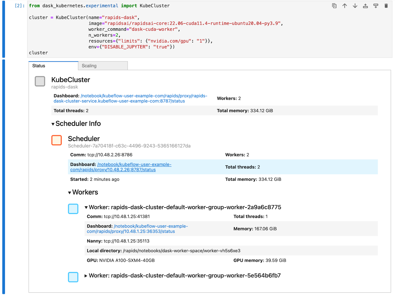
This creates a Dask cluster with two workers, and each worker has an A100 GPU the same as your Jupyter session

You can scale this cluster up and down either with the scaling tab in the widget in Jupyter or by calling cluster.scale(n) to set the number of workers (and therefore the number of GPUs).

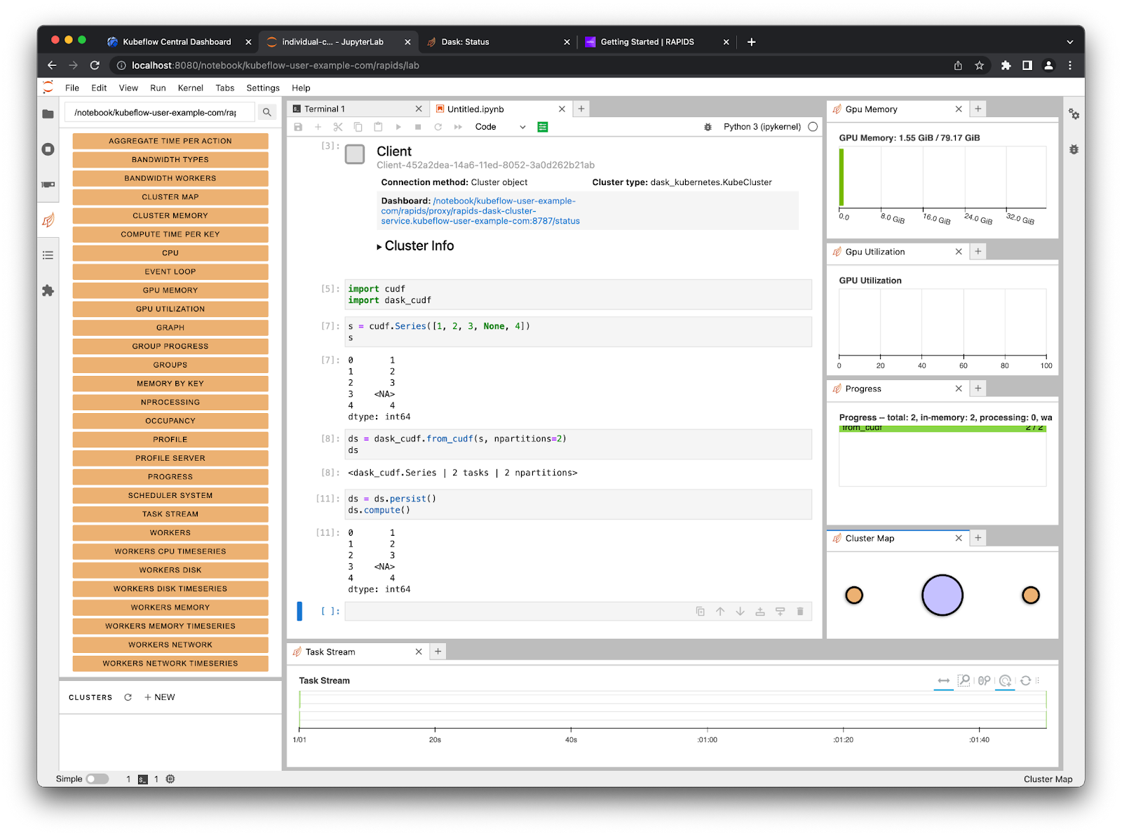
Now you can connect a Dask client to our cluster and from that point on any RAPIDS libraries that support dask such as dask_cudf will use our cluster to distribute our computation over all of our GPUs.

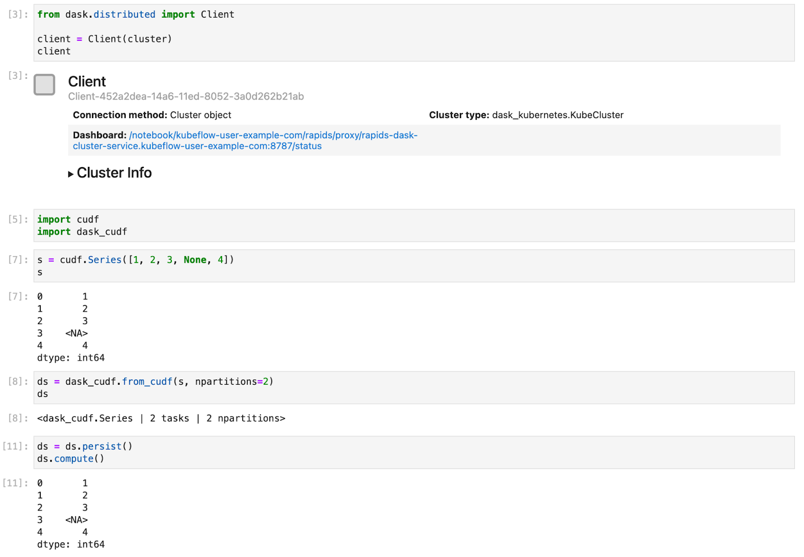
Here is a short example of creating a Series object and distributing it with Dask

Accessing the Dask dashboard from notebooks

When working interactively in a notebook and leveraging a Dask cluster it can be really valuable to see the Dask dashboard. The dashboard is available on the scheduler Pod in the Dask cluster so we need to set some extra configuration to make this available from our notebook Pod.

To do this, we can apply the following manifest.

# configure-dask-dashboard.yaml
apiVersion: "kubeflow.org/v1alpha1"
kind: PodDefault
metadata:
  name: configure-dask-dashboard
spec:
  selector:
    matchLabels:
      configure-dask-dashboard: "true"
  desc: "configure dask dashboard"
  env:
    - name: DASK_DISTRIBUTED__DASHBOARD__LINK
      value: "{NB_PREFIX}/proxy/{host}:{port}/status"
  volumeMounts:
    - name: jupyter-server-proxy-config
      mountPath: /root/.jupyter/jupyter_server_config.py
      subPath: jupyter_server_config.py
  volumes:
    - name: jupyter-server-proxy-config
      configMap:
        name: jupyter-server-proxy-config
---
apiVersion: v1
kind: ConfigMap
metadata:
  name: jupyter-server-proxy-config
data:
  jupyter_server_config.py: |
    c.ServerProxy.host_allowlist = lambda app, host: True

Create a file with the above contents, and then apply it into your user’s namespace with kubectl.

For the default user@example.com user it would look like this.

$ kubectl apply -n kubeflow-user-example-com -f configure-dask-dashboard.yaml

This configuration file does two things. First it configures the jupyter-server-proxy running in your Notebook container to allow proxying to all hosts. We can do this safely because we are relying on Kubernetes (and specifically Istio) to enforce network access controls. It also sets the distributed.dashboard-link config option in Dask so that the widgets and .dashboard_link attributes of the KubeCluster and Client objects show a url that uses the Jupyter server proxy.

Once you have created this configuration option you can select it when launching new notebook instances.

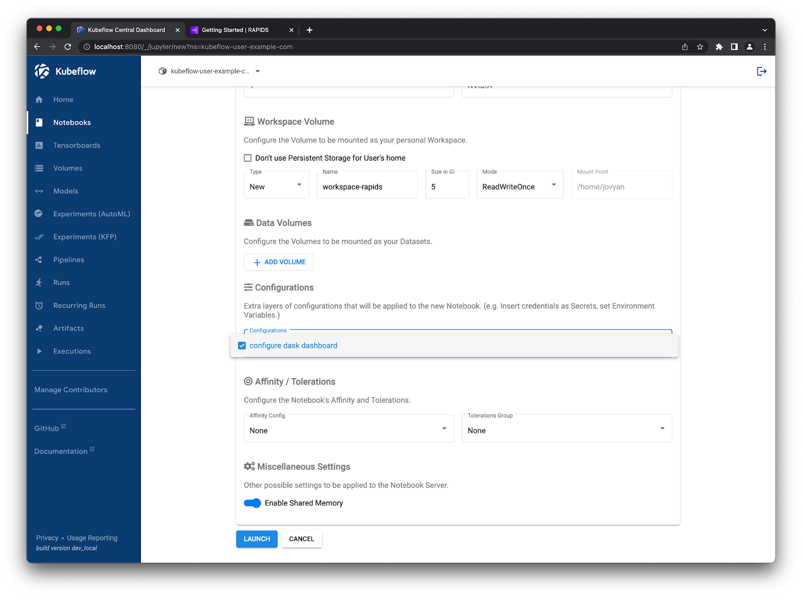
Check the “configure dask dashboard” option

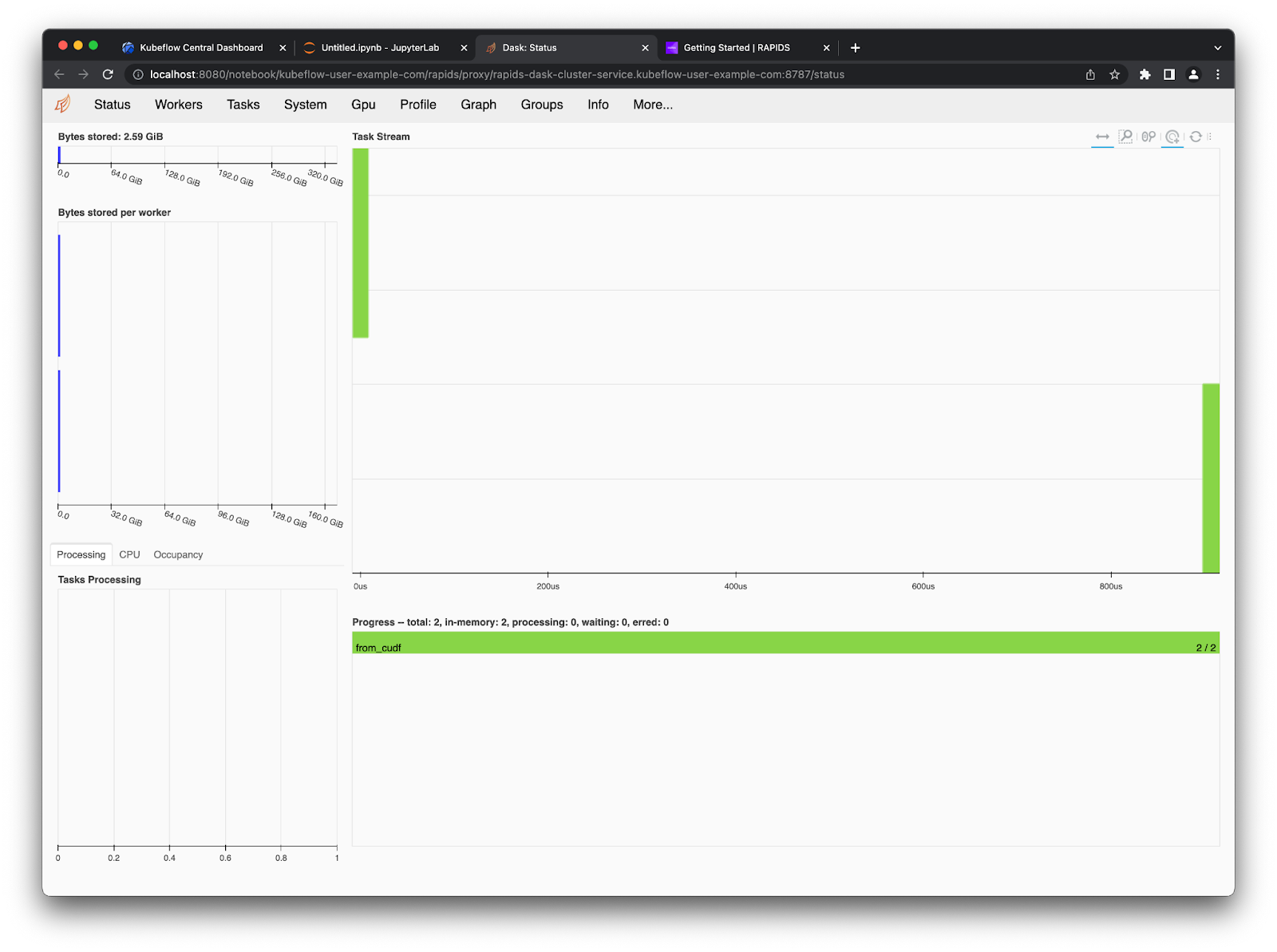
You can then follow the links provided by the widgets in your notebook to open the Dask Dashboard in a new tab.

You can also use the Dask Jupyter Lab extension to view various plots and stats about your Dask cluster right in Jupyter Lab. Open up the Dask tab on the left side menu and click the little search icon, this will connect Jupyter lab to the dashboard via the client in your notebook. Then you can click the various plots you want to see and arrange them in Jupyter Lab however you like by dragging the tabs around.